Home » All Articles
Category Archives: All Articles


RECOM – Red Cross Communications
RECOM – Red Cross Communications
About RECOM
Red Cross Emergency Communications (RECOM) was formed in 1997 and quietly built up an enviable list of achievements in technology innovation and activation service during floods, tropical cyclones and bushfires. The organisation was born out of the thoughts of a few visionary radio amateurs and the Red Cross’ Victorian Executive Director, Andrew Hilton, who had the foresight to encourage the adoption of state-of-the-art technology.
Due to the importance of the data and traffic, the design and use of a secure digital communications system was seen as imperative. RECOM developed their own suite of sophisticated software and hardware solutions for emergency deployments, whether local, interstate or overseas, based on low-bandwidth digital modes over HF amateur radio.
In fact, voice communication has never been used as the digital system is capable of transferring fully error corrected data at a useful rate when a similar power level voice signal would be totally inaudible. To make the best use of the relatively low-baud rate the data is highly compressed.
The Red Cross has activated RECOM many times over the years. During the disastrous Black Saturday bush fires in 2009 Red Cross deployed RECOM to nine evacuation centres where all communications had been lost. The data and messages from those centres were transmitted by the amateur digital HF system developed by RECOM.
RECOM field stations use an array of EMCOM Network stations for data/message delivery to clients, the Network Stations acting as digital RF to Internet Gateways. Secure messaging and file transfer (text, spreadsheets, data files and images) between field stations is also possible. The field data is presented to the “customer” via easily accessed web pages and standard email.
Deployed field stations are GPS tracked, all messages and field data GPS tagged, and all computers in the field are remotely time-locked to GPS synchronised clocks located at the EMCOM Network Stations
To satisfy the legal requirement for confidentiality when transmitting personal details of evacuees, the data is encrypted with the encryption key “rolling” after each transmission interval and time stamped and stored at the sender’s and receiver’s end for later analysis in the event of a subsequent inquest.
Nearly all members of RECOM are also members of the WIA.
Article from WIA
Emergencies and Amateur Radio
Emergencies and Amateur Radio
Introduction
In times of crisis, during both natural and man-made disasters, Amateur Radio is often used for emergency communication when landline phones, mobile phones and other conventional communications fail or are congested. Throughout history radio amateurs have made significant contributions to industry and their nations, and saved lives in times of emergency. Arthur ‘Artie’ Moore in Wales heard SOS messages from the Titanic in 1912, but was not believed, until official news of the disaster was known later.
In late March 1913, Herbert V. Akerberg, stranded for nearly 72 hours during a big flood in Ohio USA was perhaps the first person to use Amateur Radio to call for help during a disaster. Unlike commercial systems, Amateur Radio is throughout the community and not dependent on terrestrial facilities that can fail or be overloaded, such as mobile phone base sites, satellite communications links and the Internet. It can also keep going when the power grid is problematical though the use of batteries, generators and renewal energy sources. Reliable self-supported communications networks are possible to set up quickly.
Worldwide radio amateurs provide a valuable resource to Emergency Services and Aid Organisations in times of need, either by being the extra manpower required to cope with extended operations at emergency communications centres, or by facilities in the field such as equipment and infrastructure including VHF and UHF repeater systems. The range of frequencies and equipment available to them is vast, and they have specific skills in getting things to work in the most difficult circumstances, keeping them working, and getting the message through. Some explore technology, adding capabilities including the use of digital or text modes, and during an oil spill and a flood have brought responders real time vision from disaster scenes.
The United Nation’s agency, the International Telecommunications Union (ITU), has long recognised Amateur Radio as a recreation, a means of self-education and that radio amateurs can provide emergency communications. The International Telecommunications Union Development Sector (ITU-D) actively promotes Amateur Radio through its recommendation to promote “effective utilization of the amateur services in disaster mitigation and relief operations.” That means that amateur services are able to be in national disaster plans, and memoranda of understandings with amateur and disaster relief organisations are encouraged. The ITU-D revised recommendation embraces changes adopted at World Radiocommunication Conference 2003 (WRC-03) to Article 25 of the international Radio Regulations. One change is that Amateur Radio stations may transmit international communications on behalf of third parties in case of emergencies or for disaster relief. Another encourages administrations “to take the necessary steps to allow amateur stations to prepare for and meet communication needs in support of disaster relief.”
In many countries radio amateurs train to improve their skills through disaster scenarios (either alone or with other responders), field day portable operation, and routine practice at community events. They can quickly establish networks tying disparate agencies together to enhance interoperability, or stand-alone communication with message handling.
Recent Events
 |
Many recent events show the role of radio amateurs in disasters. Whether it be a seismic disturbance, adverse weather, fire, explosions or other calamity, emergency radio is there helping among many volunteers. Often severe weather occurs in South-East Asia, the Pacific, the Americas and elsewhere. Earthquakes, power outages, structure and wild fire, plus searches for missing people or injured animals, have involved emergency communications.
After a massive earthquake struck the island nation of Haiti on January 12, 2010, many individuals provided reliable local and international communications that included email, phone-patch and medical aid logistics. Other major international examples include the September 11 attacks on the World Trade Centre in Manhattan in 2001, the 2003 North America blackout, Hurricane Katrina in 2005, Hurricane Sandy in 2012, and numerous earthquakes, where Amateur Radio was used to help disaster relief activities.
The largest disaster response by the US was during Hurricane Katrina which first made landfall as it went through Miami Florida on August 25, 2005, eventually strengthening to Category 5. More than a thousand radio amateurs converged on the Gulf Coast in an effort to provide emergency communications assistance. Subsequent Congressional hearings highlighted the Amateur Radio response as one of the few examples of what went right in the disaster relief effort.
Perhaps the most destructive tsunami in history killed about 230,000 people and engulfed Indian Ocean coastal areas in 12 countries on December 26, 2004. During that disaster, communications were lost or severely disrupted. It was the ham radio operator community in many countries that helped to reunite families and assist in relief operations. A major effort in response was by the Radio Society of Sri Lanka (RSSL) that also had the world’s biggest train disaster when a train was washed off the rails at Pereliya. The RSSL was later presented with the German town of Bad Bentheim ‘Golden Antenna’ award, to recognise the use of Amateur Radio technology in connection with humanitarian work.
Among the rescue and recovery of the 2008 Great Sichuan Earthquake in the People’s Republic of China were radio amateurs, who provided emergency communications. They repeated their major effort in the devastating 2013 Ya’an earthquake. When an earthquake struck the Canterbury region in New Zealand’s South Island on February 22, 2011 radio amateurs used their emergency command van to keep rescue teams and Civil Defence staff in touch, and did a fine job among the many others involved in that disaster.
In November 2012 South African radio amateurs were asked to provide a link between Johannesburg and search teams looking for a missing aircraft in Mozambique where normal communications were not available. This was provided for four days. Community service provided in a number of countries provides emergency communication training and a time for interfacing with other responders. Such was the case on April 15, 2013 when 200 radio amateurs helping the Boston Marathon used their skills after the event was hit by bombings, to perform magnificently alongside professional first responders and medical volunteers from the Red Cross.
Typhoon Haiyan – known locally as Yolanda – struck the Philippines on November 8, 2013, and the deadliest typhoon in the country’s history. Over 14 million people were affected across 46 provinces. The City of Tacloban, home to 220,000 people, suffered more loss of life than any other area. Throughout the disaster area the government put the loss of life at 6,201 and many people are missing. An estimated 100 radio amateurs provided emergency communications in response to the disaster and worked with other agencies for many weeks.
A winter storm in Slovenia in February 2014 caused the loss of power to 25 per cent of the country and European Union support mechanisms to be triggered to provide electricity generators. At the request of the Austrian Fire service, a communications link was provided between Austria and Slovenia for 10 days to ensure reliable communications between the Austrian team and their home base.
The Australian Scene
 |
Exactly when radio amateurs in Australia first assisted the community or government authorities is still unknown. However, we do know that a tropical cyclone in the Cairns area of North Queensland in February 1927 had cut all communications. Andy Couper 4BW in North Queensland and Leighton Gibson 4BN in Brisbane handled press traffic then were allowed private messages for five days during the disaster.
It is a tradition in Australia for radio amateurs to provide communications for the community during cyclones, fires and floods. Amateur Radio notably handled emergency communications for the 1939 Black Friday bushfires, Cyclone Tracy in Darwin 1974, Ash Wednesday bushfires 1983, the Newcastle Earthquake 1989, and the Black Saturday disaster in February 2009. There have been numerous other rescues and searches. Earthquakes are unusual in Australia, but on December 28, 1989 the town of Newcastle, New South Wales, was rocked by an earthquake that killed 13 people and made over 15,000 homeless.
Also through WICEN, emergency services were also provided during the 1994 and 2002 Sydney Bushfires. Extreme alpine forest fires in southeast Australia in January and February 2003 again saw radio amateurs providing emergency communications and winning high praise for their efforts.
Again radio amateur repeater facilities were used for emergency service communications during the disastrous Queensland floods in January 2011. WICEN was again effective during the Tasman Peninsula fires in January 2013.
A turning point occurred in Victoria with the Ash Wednesday 1983 disaster resulting in the emergency communications service of WICEN gaining greater recognition by government and other players in emergency response and recovery. It presented to and was featured in the Miller Inquiry into that disaster. Then greater communications resources were made available by government to emergency services, while the universal availability of mobile phones and other factors began to play. By the early 1990s there were doubts that Amateur Radio would ever again play a significant emergency communications role.
However, in 1997 the Red Cross Emergency Communications (RECOM) was formed by a group of radio amateurs using digital amateur radio and quietly built up an enviable list of achievements. During the disastrous Black Saturday bushfires in 2009 the Red Cross deployed RECOM to nine evacuation centres, where all communications had been lost.
The data and messages from those centres were transmitted by the Amateur Radio digital HF system developed by RECOM. Following the 2009 Black Saturday bushfire disaster it became evident that the needs of Emergency Service Organisations (ESOs) and Non-Government Organisations (NGOs) had changed over the previous couple of decades.
WICEN also had a role to play in Black Saturday gaining some high level recognition for its work. Coupled with the demonstrated rapid and pre-planned response of telecommunications companies to maintain or quickly restore telephone services in the bushfire affected areas, electricity supply companies also restored power within relatively short timeframes.
Modern emergency communications infrastructure is now more robust and reliable, in some cases allowing seamless communications between various ESOs over the Government Radio Network. Mobile phone network coverage is also robust and extensive however these more complex systems are still vulnerable to disasters which may cut their power supplies. So there is always a need for trained and adaptable radio amateurs, sometimes providing their own equipment and skills, but also to be trained in other important counter-disaster work. They are trained and prepared for any emergency communication call that can vary among many regional WICEN groups depending on their local needs.
Conclusion
Most of the time modern communications work well. Despite the development of very complex systems – or maybe because they are so complex – Amateur Radio has been called into action again and again round the world to provide communications when it really matters.
Amateur Radio – A Trusted Partner in Emergency Response.
Article from WIA


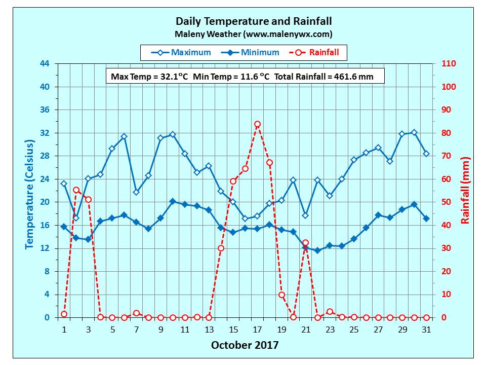
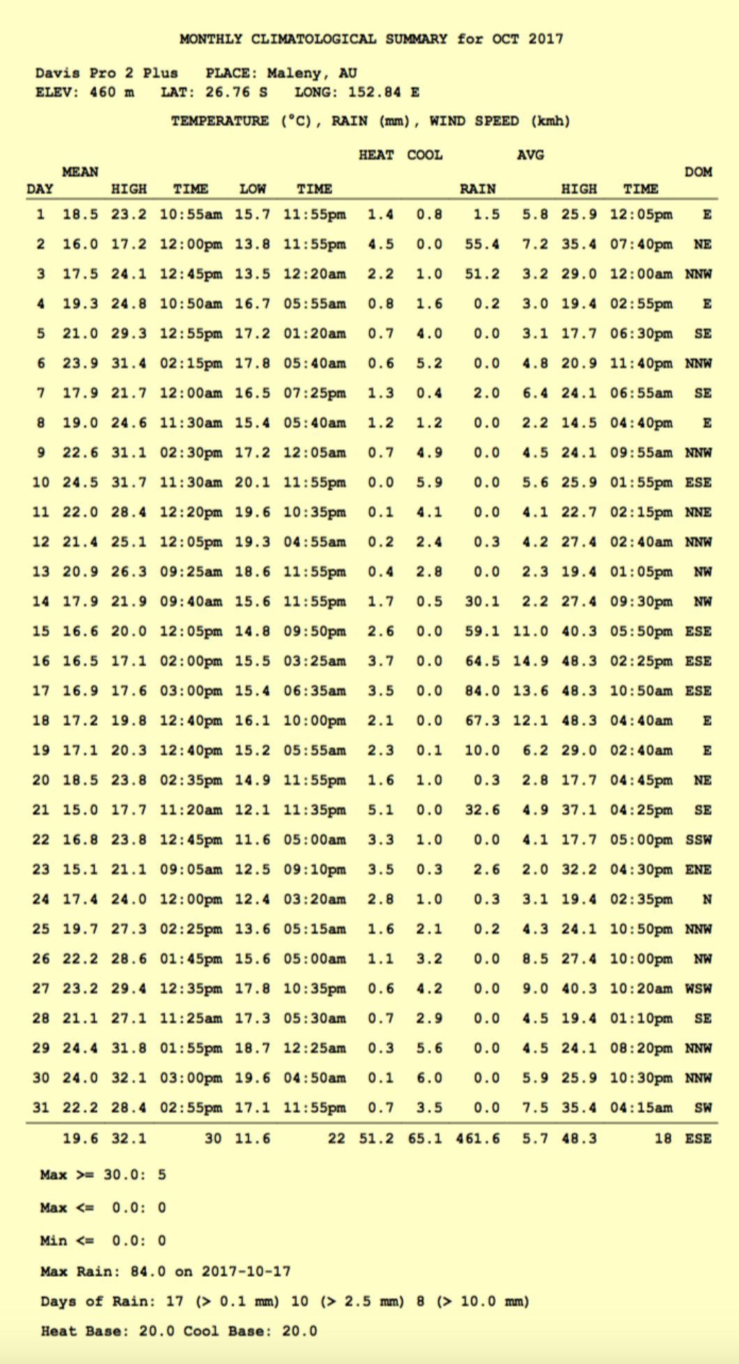
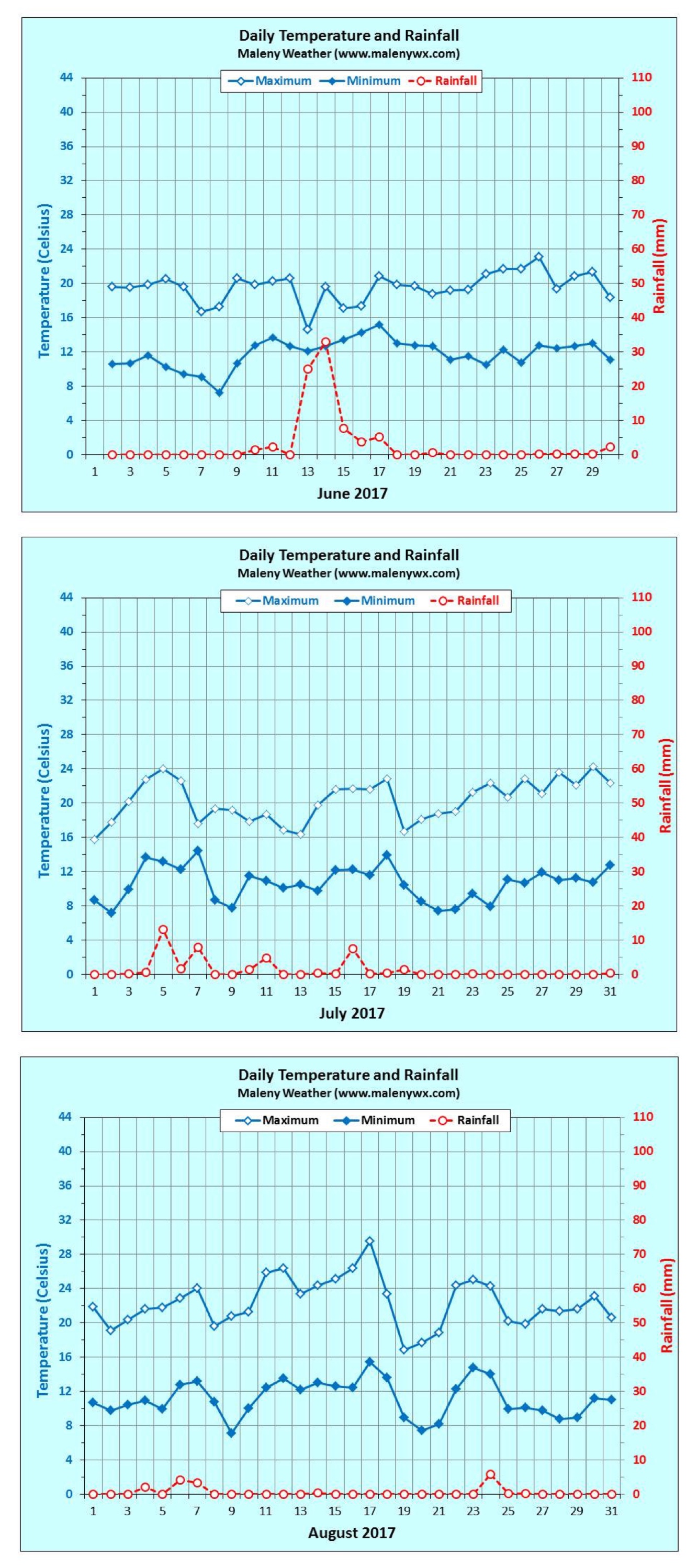
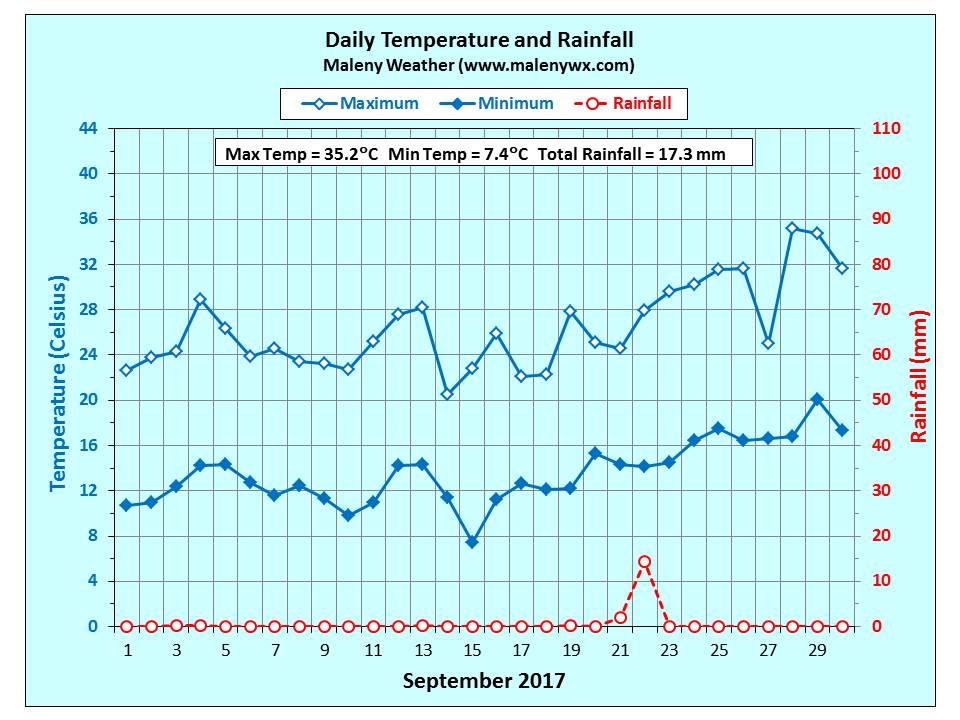
Seasonal Graphs – Spring 2017


Understanding Fire Weather
Understanding fire weather
05 September 2017
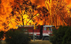
Weather conditions influence the size, intensity, speed and predictability of bushfires—and how dangerous they can be. Large fires can even create their own weather. Understanding fire weather and the peak bushfire seasons across Australia means you can be better prepared for this hazard.
When is fire season?
In Australia, the likelihood of a fire occurring at certain times of year varies by area—but the reality is that fires can happen at any time of year, driven by local conditions.
For northern Australia, the peak bushfire period is during the dry season, which is generally throughout winter and spring. For southern Australia, the bushfire season peaks in summer and autumn.
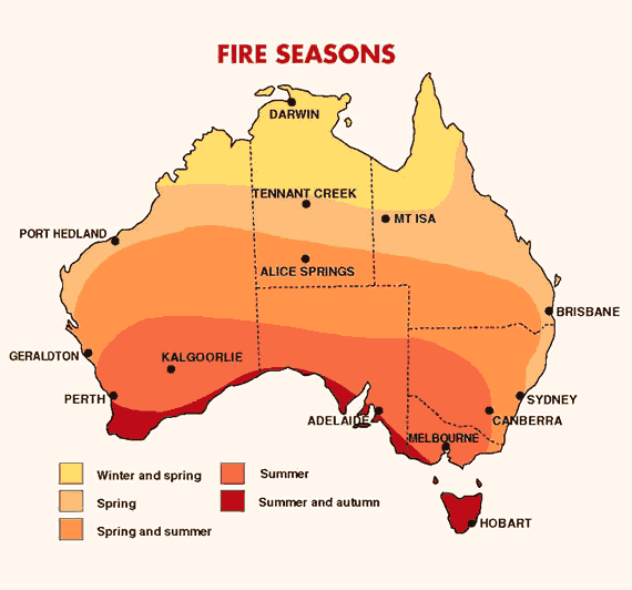
Image: fire seasons in different parts of Australia
What factors influence fire behaviour?
Weather-related factors that contribute to an increased risk of bushfire danger include:
- high temperatures;
- low humidity;
- little recent rain;
- abundant dry vegetation;
- strong winds; and
- thunderstorms.
When the weather is hot, humidity (moisture in the atmosphere) is low and there’s been little recent rain, vegetation dries out and becomes more flammable. Periods of wet weather can encourage vegetation growth, increasing the amount of fuel available—and future bushfire risk, if dry weather follows.
Strong, gusty winds help fan flames and will cause a fire to spread faster across the landscape, reducing the time you have to prepare.
Above the fire, strong winds can carry hot embers long distances. These can start ‘spot’ fires many kilometres ahead of the main fire front.
A change in wind direction can bring a dangerous period of bushfire activity. This is often seen as a trough or cold front (also known as a cool change) shifting the direction of the wind, altering the course of the fire and broadening the fire front.
Lightning, produced by thunderstorms, can ignite bushfires. Large fires can also create their own thunderstorms. These are known as pyrocumulonimbus, and are caused by the heat of the fire forcing the smoke and hot air above it to rise to the point where it cools and condenses into water droplets, eventually forming large clouds. Pyrocumulonimbus can cause erratic, more intense and dangerous bushfire behaviour, including lightning strikes that can cause new fires.
Fire warnings
The Bureau issues fire weather warnings when forecast weather conditions are likely to be dangerous. We work closely with emergency services around the country to keep the community informed.
The Bureau and emergency services use six fire danger ratings to communicate the level of bushfire risk. These ratings help the community know when to put their bushfire survival plan into action.
These ratings are: Low–Moderate, High, Very High, Severe, Extreme and Catastrophic (or Code Red in Victoria). The higher the rating, the more dangerous the conditions are likely to be, and at higher ratings any fire that starts will likely be fast-moving and difficult to control.
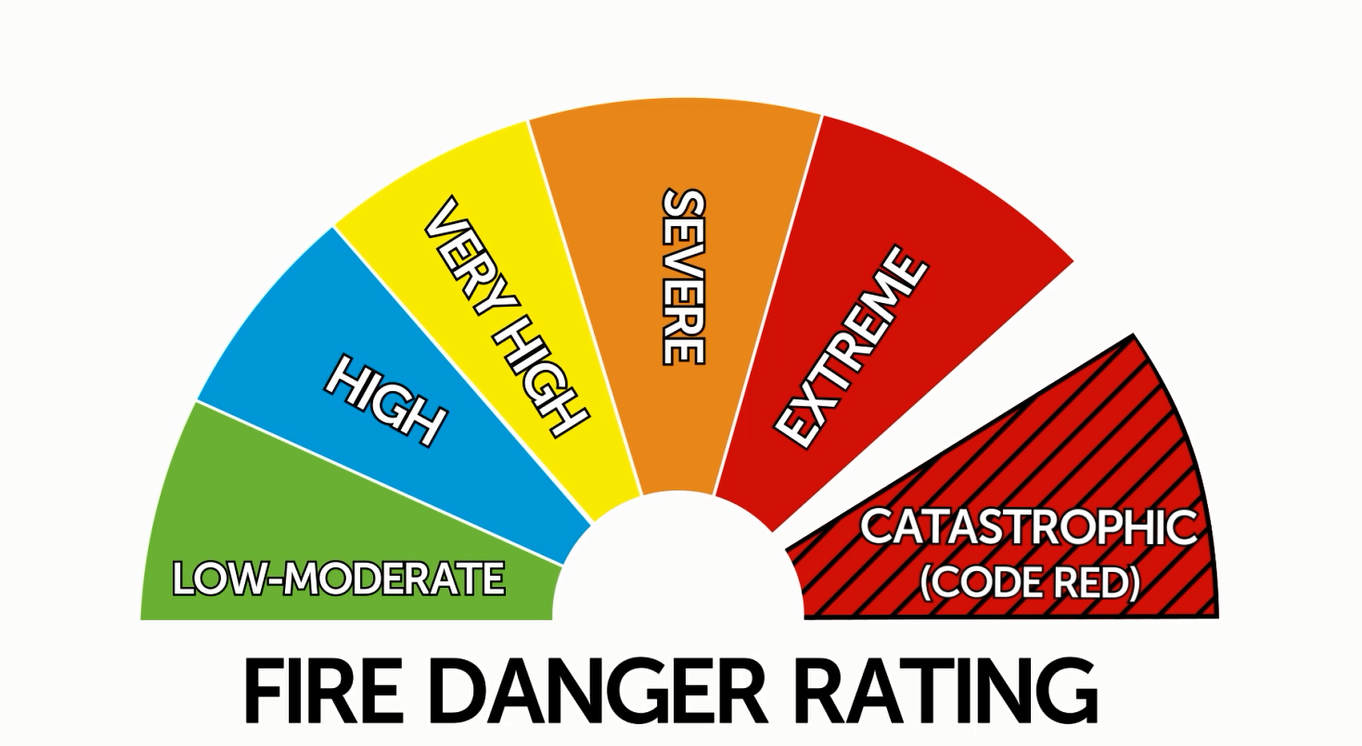
Image: Fire danger ratings used in Australia
What to do when there’s a risk of fire
No matter what the forecast fire rating, if you live in or are travelling to an area that could be threatened by fire, you need to have a bushfire plan in place, so you know what to do if a bushfire starts. On a day when dangerous bushfire activity is more likely, stay in touch with your local fire agency and emergency services via their websites and social media—and tune into emergency broadcasters.
More information
- Fire weather warnings
- Access all current warnings on our website (select your State or Territory and ‘View the current warnings’) or the BOM Weather app (tap the yellow triangle with the exclamation mark). You can also follow your State/Territory’s handle on Twitter.
- Bushfire weather
- Research: how mountain waves can escalate bushfires


Long and Short Waves
Long and Short Waves
Long Waves
The hemispheric weather patterns are governed by mid-latitude (23.5°N/S to 66.5°N/S) westerly winds which move in large wavy patterns. Known as planetary waves, these long waves are also called Rossby waves, named after Carl Rossby who discovered them in the 1930’s.

Rossby waves form primarily because of the earth’s geography which does two things. First, the earth’s heating from the sun is uneven due to the different shapes and sizes of the land mass (called differential heating of the earth’s surface). Second, the air can’t travel through a mountain so it must rise up and over or go around.In both cases, the disruption of the air flow creates imbalances in temperature distribution both vertically and horizontally. The wind responds by seeking a return to a “balanced” atmosphere and changes speed and/or direction. However, as long as the sun keeps shinning, those imbalances will continue to develop. Thus the wind will constantly be changing directions, and develop into wave-like patterns.
The length of long waves vary from around 3,700 mi (6,000 km) to 5,000 mi (8,000 km) or more. They generally move very slowly from west to east. But occasionally they will become stationary or retrograde (move east to west).
The speed at which these large waves move should not to be confused with the speed of the wind found within the waves themselves. For example, there can be a strong jet stream wind of 100 kts (115 mph / 185 km/h) moving through the long wave but the position of long wave itself move may very little. The wave itself is not moving at 100 kts, just the wind within.
Rossby waves help to transfer heat from the tropics toward the poles and cold air toward the tropics trying to return the atmosphere to balance. They also help locate the jet stream and mark out the track of surface low pressure systems. The number of long waves at any one time varies from three to seven though it is typically four or five.
Their slow motion often results in fairly long persistent weather patterns. For example, locations between the trough and the downstream ridge can experience extended periods with rain or snow while at the same time 1,500 – 2,000 miles (3,000 – 4,000 km) upwind and/or downwind the weather is very dry.
This often can lead to a misconception where one assumes the weather he or she experiences is typical everywhere. That is simply not true. If one place is receiving cooler weather and/or flooding rains over a period of several days to weeks, then there are some other places where the weather is warm and dry for about the same period. It all depends upon the location of the long waves relative to the observer.
Short Waves
A “piece of energy”, “vort max” (or “vorticity maximum”), “pocket of cold air” (or “pocket of energy”), “upper level disturbance”, “upper level energy”, or just “shortwave” are some of the slang terms for waves with a length of less than 3,700 miles (6,000 km).
They are embedded within the long waves and move much faster and throughthe long waves. Unlike the slow movement of long waves, short waves move east (down stream) on average of 23 mph (20 kts, 37 km/h) in summer and 35 mph (30 kts, 55 km/h) in winter. This motion causes long waves to distort and change shape such as deepening long wave troughs and flattening long wave ridges.
Due to their variety of sizes, it can be difficult to discern short wave embedded within a long wave by looking at a static map. One often needs to see looping images of the wave patterns to determine the difference between them.
Short waves, embedded within long waves, are also the chief instigator of episodes of precipitation. Main precipitation bands will be typically localized near the short wave as it passes overhead.
Below is an example of a 500 mb chart. The height contours are in black. The brown arrows indicate direction of airflow. The large red dashed lines represent the location of the long wave troughs.

The shorter blue dashed lines represent the location of the of the more prominent short waves. (There are more short waves than indicated.) The green areas represent precipitation totals. The areas of precipitation are mainly associated with the short waves as they pass through the long waves. Like cars on a train tack, short waves will generally follow height contours.
Constant Pressure vs. Constant Elevation
Constant Pressure vs. Constant Elevation
Both at the surface and in the upper atmosphere, meteorologist constantly refer to “high” and “low” pressure systems. However, we look at them from two different perspectives.At ground level, we seek air pressure values as they relate to “sea level” which provides us with a picture of the weather patterns at the surface. Using sea level (elevation = zero) as the common baseline we are able to make meaning of different pressure values between stations. So, on all surface charts, the elevation of the “surface” is considered zero feet.
The lines drawn on surface charts connecting areas of equal pressure are called isobars. “Iso” means equal and “bar” is the unit by which we measure pressure. Therefore, an isobar is a line representing the location where the pressure is equal (the same) along that line.

When we examine the atmosphere however, since air pressure decreases with increasing altitude, the elevation at which any particular pressure value occurs will vary from reporting station to reporting station.
These changes in elevation represent different densities (and ultimately air temperature) in the atmosphere. The height of any pressure level is determined by the density of the air. As the air temperature decreases the air’s density increases.
Therefore, the altitude where any particular pressure occurs will be lower in the atmosphere is regions of colder air. Conversely, higher air temperatures result in lower densities with the corresponding altitude of various pressure levels higher.
This is why, as a rule, the altitude of constant pressure levels decrease from the equator toward the poles simply because it is colder at the poles than at the equator.
Therefore, we look at the atmosphere at fixed pressure levels and see the altitude at which these specific pressure levels occur. So for upper air weather maps, instead of looking at the pressure at the sea level elevation, we look at the altitudes at which constant pressures occur.
The lines drawn on constant pressure charts are called isoheights, lines of equal height. For example, on the 500 millibar pressure chart, the air pressure is a constant 500 millibars all across the map. Therefore, the lines on that chart represent the altitude at which the air pressure of 500 millibars was reached. In essence, upper air charts show the atmosphere in three dimensions.
By convention meteorologists simply refer to isoheight lines as ‘contours’. By looking at these contours we observe the upper air weather patterns such as ridges of higher heights and troughs of lower heights. And it is these ridges and troughs that govern the weather we experience at the surface.
Analogous to topographic charts, ridges are areas where the elevation of any particular pressure value is higher than the surrounding heights of that same pressure value. And troughs are like valleys in that they lie along areas of the lowest elevations of any particular pressure value.

Introduction to Upper Air Charts
Introduction to Upper Air Charts
One of the first things to always keep in mind is weather is like the humidity, its all relative. In some aspects, absolute values of pressure and temperature are not as important as the change in pressure or the change in temperature. In meteorology, we refer to the “change in” as a gradient.

Any time there is a rapid “change in” any particular weather element we will say the “gradient” is large. It is near these large gradients where the weather is most active.A common example is found near cold fronts. The “change in” air pressure is typically rapid near a cold front and therefore the pressure “gradient” is large. The greater the pressure gradient is near a front the stronger the wind. This is just as true for the upper atmosphere.
While the information a skew-t chart provides is invaluable, it will only tell us what is happening in the atmosphere at that location. To paint a complete picture of the atmosphere as a whole we need to view radiosonde data from many upper air observations.
We do this by creating constant pressure charts that let us see changes, and gradients, in atmospheric conditions across the country and around the world.
The Air Up There: Skew-T Examples
The Air Up There: Skew-T Examples
Radiosonde observations provide the condition of the atmosphere above the launch site (typically within 25 miles/40 km) at the time of launch. While they do not provide any direct forecast information, they do help explain why we experience different types of weather. Following sample soundings are typical for different weather conditions.
Snow
The atmosphere is very moist as indicated by the small amount of separation between the air temperature (red line) and the dew point (blue line). Even though the air temperature increases a few hundred feet above the ground (a temperature inversion) the air temperature, throughout the entire atmosphere, remains below freezing.
So, when precipitation begins, it will be in the form of snow and will remain frozen as snowflakes reaching the ground.

Ice pellets (Sleet)
As with the previous sounding, the atmosphere is very moist. So much so, the air temperature and dew point are the same from near 900 millibars (3,000 ft. / 1,000 m) to a little above 700 millibars (10,000 ft. / 3,000 m).
At the surface, an arctic cold front had moved south of the observation station with an air temperature well below freezing. The air temperature begins to decrease with height (which is normal) dropping from 23°F to 12°F (-5°C to -11°C).
However, the density of the arctic air is such that it lays close to the ground with its vertical extent fairly small, in this case only about 3,000 feet (1,000 meters) deep. Above 900 millibars (3,000 ft. / 1,000 m) the air becomes considerably warmer. This area is called an inversion, where temperature change with height is ‘inverted’ as it increases with height instead of typically decreasing with height. This inversion is often also referred as a ‘warm nose’.
Eventually, the temperature of the atmosphere will return to the typical decrease with height (near 800 mb) and will continue to cool until it falls to below freezing again (about 720 mb).
While there may be some precipitation forming as rain in the warm ‘nose’ region where the air temperature is above freezing, the vast majority of precipitation will form as snow in the colder below freezing air above the inversion.
As snow falls into the ‘warm nose’, it melts into a liquid drop/rain. Then the liquid drops fall back into the arctic air mass (near the ground) that is cold enough and deep enough for the liquid to freeze into ice pellets before reaching the ground.

Freezing Rain
The basic pattern for freezing rain is similar to ice pellets. The main difference is the cold, dense air near the surface is very shallow and/or the ‘warm nose’ is large or very warm or both. The melted snow does not have sufficient time to freeze before is reaches the ground.
Therefore, precipitation falls as rain but then it freezes upon contact with a surface such as a tree, power line, automobile or bridge. As a general rule, elevated surfaces will ice first because the ground cannot keep them warm, allowing them to cool to the air temperature quickly. This allows the rain to freeze to ice on contact with these surfaces.
Elevated surfaces may be capable of accumulating ice as soon as the air temperature falls below 32°F (0°C). Road surfaces in contact with the ground will generally begin to ice when the air temperature falls to 28°F (-2°C).

Hurricane
Inside hurricanes, the velocity of the air helps keep the air mixed. Therefore, other than the normal decrease with height, variations in temperature (and dew point) are fairly minimal.

Skew-T Plots
Skew-T Plots
As the radiosonde balloons ascends, it records the temperature and relative humidity at certain prescribed pressure levels (called the mandatory levels) and anytime a significant change occurs in the temperature, humidity, or wind.
Typically, a radiosonde observation is complete when the balloon, carrying the radiosonde, bursts and begins to descend. At that time the data is compiled into a series of five-digit groupings containing temperature, dew point depression and wind speed/direction for mandatory and significant levels. This data is plotted onto a skew-T.
The five-digit coded radiosonde observation is complicated to decode and plot onto a Skew-T diagram. As such, there are several private weather vendors and universities who have written programs to decode and plot (or redisplay the info in a tabular format) these observations. A simple Internet search for “atmospheric soundings” will provide you with several choices.
There are two basic lines plotted on a Skew-T from which we can derived much information. These represent the dew point which is calculated from the relative humidity (in blue, left line) and air temperature (in red, right line).

While it is generally true that the air temperature decreases with height, it is readily seen that this decrease is not uniform nor is it consistent. There may be several places where the air temperature remains the same or increases with height. These particular places are called ‘temperature inversions’ where the normal temperature decrease is ‘inverted’ and the temperature will increasewith height.
Another common characteristic of radiosonde soundings is the location of the tropopause. The tropopause is the boundary between the troposphere and stratosphere and is also indicated by a large temperature inversion.
The dew point line will be the most ‘wiggly’ as the radiosonde ascends through intervening pockets of moist and dry air. At each level on the Skew-T, the closer the dew point is to the temperature, the higher the relative humidity is at that level. The dew point will occasionally equal the air temperature and will be seen by the intersection of both lines.
The other piece of information plotted on a Skew-T is the wind speed and direction. This info obtained as the radiosonde is tracked using GPS during its ascent. The wind speed and direction is reported for the same mandatory pressure levels with additional required elevations above sea level and for any significant changes in speed or direction.
Across the country and around the world, radiosondes sample the atmosphere twice daily providing answers concerning the state of the upper air.

Skew-T Log-P Diagrams
Skew-T Log-P Diagrams

Once the radiosonde observation is plotted, the Skew-T will show the temperature, dew point, and wind speed/direction. From these basic values a wealth of information can be obtained concerning the meteorological condition of the upper air.
There are six basic set of fixed lines that comprise the skew-t diagram. (You can toggle on/off each of these lines on the image at bottom.)
- Temperature
- Temperature lines are drawn at a 45° angle with temperature values that increase from the upper left to the lower right corner of the chart. Early versions of this upper air chart were made with the temperature lines drawn in the vertical.
But in 1947, the modification of tilting the temperature lines 45° aids in analysis. This is where the name “Skew-T” comes from as the temperature lines are skewed at a 45° angle.
- Pressure
- Pressure lines are drawn in the horizontal. Distance between the lines increases from the bottom to the top of the chart (1050 millibars) to the top (100 millibars). This is due to the decrease in atmospheric density with increasing elevation (Learn more about atmospheric density).
Atmospheric pressure decreases logarithmically with increasing elevation. Therefore the heights of the various pressure levels are plotted as the “log” of the pressure…”Log-P” portion of the Skew-T Log-P diagram.
- Dry Adiabats
- Slightly curved, these lines increase in value (°C) from lower left to upper right. Dry adiabats represent the rate at which UN-saturated air cools as it rises. (Unsaturated air is air with a relative humidity lower than 100%.) As unsaturated air rises, it expands and cools with the temperature decreasing (or lapses) at a rate of 9.8°C per 1000 meters (5.5°F/1000 feet) until the relative humidity becomes 100% (the air becomes saturated). This rate is called the “dry adiabatic lapse rate” and these lines on the Skew-T represent that value.
- Moist (or Saturated) Adiabats
- These curved lines increase in value (°C) from left to right. Moist adiabats represent the rate at which saturated air cools (lapses) as it rises. When the air is at 100% relative humidity, further cooling causes water vapor to condense.In this condensation process, heat is released which then affects the rate of cooling and these lines represent that rate.
Near the surface, as saturated air rises, it expands and begins to cool at a rate of about 4°C per 1,000 meters (2.2°F/1,000 feet). As it continues to rise, the cooling rate decreases due to a decreasing amount of water vapor.
On the Skew-T the dry and wet adiabats become nearly parallel in the upper troposphere where the rate of cooling approaches that of dry adiabats, nearly 9.8°C/1,000 meters (5.5°F/1,000 feet).

Very cold air does not contain much water vapor. The reason is because as air cools, the temperature of the water vapor itself decreases leading to an increasing amount vapor condensing to a liquid (or deposits to a solid) state. This condensation and/or deposition decreases the amount of gaseous water remaining in the atmosphere.
With very cold air most of the water vapor has already condensed into a liquid or deposited into a solid. The end result is very cold air contains little water vapor and therefore cannot release much heat into the atmosphere.
Conversely, very warm air can contain large amounts of water vapor. Warming air means the temperature of the water vapor increases so evaporation and/or sublimation (changing from liquid or solid to a gas) also increases. This adds water vapor to the atmosphere.
In the tropics, the large amount of heat released by process of condensation from very moist air is one of the mechanisms for the formation of tropical cyclones and thunderstorms.
- Mixing Ratio
- In meteorology, mixing ratio is the mass of water vapor compared with the mass of dry air. It is expressed in grams per kilogram. Two mixing ratios can be learned from a Skew-T, the ordinary mixing ratio and the saturation mixing ratio. On a plotted radiosonde sounding, the mixing ratio at any given level is the amount of water vapor in the air where the dew point temperature line crosses the mixing ratio line.
The saturation mixing ratio is the maximum amount of water vapor that can be in the air at any given level and is found where the temperature line crosses the mixing ratio line.
- Wind Staff
- These staffs are for plotting the wind speed and direction as observed by the radiosonde.
Radiosondes
Radiosondes

Since the weather we experience is due to dynamic processes that take place throughout the atmosphere, we need to know what is taking place through the entire atmosphere. These observations are primarily taken with the aid of radiosondes.The radiosonde is a small, expendable instrument package that is suspended below balloon filled with either hydrogen or helium. As the radiosonde rises, sensors on the radiosonde measure values of pressure, temperature, and relative humidity.
These sensors are linked to a battery powered radio transmitter that sends the sensor measurements to a ground receiver. By tracking the position of the radiosonde in flight via GPS (global positioning system), information on wind speed and direction aloft is also obtained.
Worldwide, most radiosonde observations are taken at 00Z and 12Z daily (What is ‘Z’ time?). With worldwide coordination of these upper air observations we can get a good picture of the various pressure and wind patterns across the globe. For the United States mainland observation sites, the local times for these observations are centered around 6 AM and 6 PM daily.
Technically, a radiosonde observation provides onlypressure, temperature, and relative humidity data. When the position of a radiosonde is tracked (so that wind speed and direction can be determined) it is called a rawinsonde observation.Most stations around the world take rawinsonde observations. However, meteorologists and other data users frequently refer to a rawinsonde observation as a radiosonde observation.
The radiosonde flight can last in excess of two hours, and during this time the radiosonde can ascend to over 115,000 feet (35,000 m) and drift more than 125 miles (200 km) from the release point. During the flight, the radiosonde is exposed to temperatures as cold as -130°F (-92°C) and air pressure of only a few hundredths of what is found on the Earth’s surface.
When the balloon has expanded beyond its elastic limit (about 20 feet in diameter) and bursts, the radiosonde returns to Earth via a small parachute. This slows its descent, minimizing the danger to life and property.
If found, radiosondes can be reconditioned and used again saving the taxpayer some money. If you find a fallen NWSradiosonde, it is safe to handle. Cut the string to the burst balloon and place it in a trash receptacle.

Next, remove the plastic mailbag attached to the handle of the radiosonde and place the instrument inside the bag. Hand the package to your postal carrier. Postage is prepaid if the instrument is returned in the United States.Worldwide, there are about 1,300 upper-air stations. Observations are made by the NWS at 92 stations – 69 in the conterminous United States, 13 in Alaska, nine in the Pacific, and one in Puerto Rico.NWS supports the operation of 10 other stations in the Caribbean. Through international agreements data are exchanged between countries worldwide.
How Are Radiosonde Data Used?
Radiosonde observations are used over a broad spectrum of efforts including:
- Input for computer-based weather prediction models,
- Local severe storm, aviation, and marine forecasts,
- Weather and climate change research,
- Input for air pollution research, and
- Ground truth for satellite data.
Data from a radiosonde observation is plotted on a seemingly complicated chart called a “Skew-T” but provides is a wealth of information concerning the state of the atmosphere.
Stability/Instability
Stability/Instability
The following ball and bowl illustrations should help in understanding parcel stability and instability. The bowl represents the ‘state’ of the atmosphere. The red ball represents a “parcel” of air upon which an energy is applied to the ball to initiate motion.
Absolute Stability
With the ball inside of the bowl it will return to its initial position. In the atmosphere, if a parcel returns to its initial starting elevation then the atmosphere is considered to be absolutely stable.


Absolute Instability
With the bowl turn upside down, the ball now rests on the top of the bowl. When a force is applied to the ball it begins to move on its own without any additional force applied. When this occurs in our atmosphere it is considered absolutely unstable.


Neutral Stability
On a flat surface, it a force is applies to the ball it moves. Once the force is removed the ball stops and remains in its new position. In the atmosphere, the atmosphere this considered neutral stability.


Conditional Instability
The upside down glass bowl has a slight depression wherein the ball rests. If the force is not too great the ball will return to its initial position similar to absolute stability. However if the force is strong enough the ball will move up and out of the depression and continue to move on its own. This is one of the most common states of the atmosphere called conditional instability. The atmosphere is unstable if certain conditions are met otherwise it is stable.


To measure the state of the atmosphere over our heads (temperature profile, stability, moisture, wind, etc.) we use a device called a radiosonde.
The ‘Parcel’ Theory
The ‘Parcel’ Theory
It is common knowledge that warm air rises. It is normally assumed that is because warm air is lighter than cooler air. While that is true there is a more fundamental process that takes place for the cause of rising warm air.

Warm air rises primarily due its lower densityas compared to cooler air. As the temperature increases, the density of the air decreases. But even air that is of a lower density will not begin to rise by itself.Isaac Newton’s first law of physics is that the velocity of an object will remain constant unless another force is exerted on that object. The more common way of saying this is ‘an object at rest tends to stay at rest and an object in motion tends to stay in motion’.
This is why decreasing the density of air alone is not sufficient enough to cause air to rise. There must be another force exerting on the less dense air for it to begin its upward motion.
That force is ‘gravity’. Gravity’s role is its pull of cooler, denser air toward the earth’s surface. As the more dense air reaches the earth’s surface it spreads and undercuts the less dense air which, in turn, forces the less dense air into motion causing it to rise.
This is how hot air ballooning works. A flame is used to heat the air inside of the balloon making it less dense. Outside of the balloon, the cooler air, being more dense, is pulled towards the earth’s surface by gravity. The cooler air undercuts the warmer, less dense air trapped inside the balloon causing it to lift.
This is why thunderstorms often form along weather fronts. A front represents the boundary where cooler, more dense air undercuts less dense, warmer air forcing it up into the atmosphere forming the storms.
In meteorology, we often treat ‘pockets of air’ in a similar way to ballooning. We call these pockets of air “parcels”. A parcel is a bubble of air of no definite size that we generally assume it retains its shape and general characteristics as it rises or sinks in the atmosphere.
The theory behind the “parcel” has several assumptions.
-
In a stable atmosphere, the rising parcel becomes cooler than the surrounding environment slowing or ending its rise (left image). In an unstable atmosphere, the temperature of the parcel is higher than the surrounding environment and as such remains buoyant and will continue to rise (right image).
In both cases the parcel’s rate of cooling remains fixed. Therefore, stability/instability is based upon the vertical temperature profile of the atmosphere.We generally assume the ratio of moist air to dry air in the parcel remains constant as it rises (or sinks) in the atmosphere.
- We also assume there is no outside source of heating added to the parcel.
- Any parcel that is UNsaturated (relative humidity less than 100%) will cool (or lapses) at a rate of of 9.8°C per 1,000 meters (5.5°F/1,000 feet) until the relative humidity becomes 100% (the air becomes saturated).
- Any saturated parcel (parcel with 100% relative humidity) cools at a slower rate. This is because the process of water vapor condensing into a liquid releases heat. The released heat that is added to the atmosphere slows the rate of cooling.

Because of many different influences on a parcel of rising air most, if not all, of the assumptions will not be 100% true at all times. However, the ‘parcel theory’, while an over-simplification of real world processes in the atmosphere, is a good way of thinking about how the atmosphere produces the weather.
Buoyancy: Positive and Negative Energy
The reason for looking at parcels is to help determine the stability of the atmosphere. As an unsaturated parcel rises it will cool at the fixed rate of 9.8°C per 1,000 meters (5.5°F/1,000 feet).
If the temperature of the rising parcel decreases to less than the surrounding atmosphere (due to its cooling) the parcel will become denser than the surrounding environment and gravity will slow, or even reverse, the rise. This is called negative energy and means the atmosphere at that level is ‘stable’.
If the temperature of the rising parcel remains higher than the surrounding atmosphere (despite its cooling), the parcel, being less dense than the surrounding environment, will continue to rise. This is called positive energy and means the atmosphere at that level is ‘unstable’.
Introduction to the Upper Air
Introduction to the Upper Air
What we experience as weather at ground level is the end result of what takes place over our head. Therefore to determine the forecast, and therefore the impacts, of weather we will need to determine the weather patterns in the upper air before looking at the surface weather.

The term “upper air” refers to the earth’s atmosphere above about 5,000 feet (1,500 meters). It is from the upper air where we get our rain and drought, wind and calm, heat and cold at the earth’s surface.
The map (above) was a picture the state of the atmosphere for a particular time at about 18,000 feet in altitude. The lines represent the locations of various higher and lower pressure regions in the upper atmosphere.
While upper air maps like this (and following information) can be rather complicated, this is the “meat and potatoes”‘ for the meteorologist.
All weather forecasts stem from our understanding of the upper air where weather patterns such as ridges, troughs, upper air disturbances and upper-lows occur and where they are moving.
The Color of Clouds
The Color of Clouds
The color of a cloud depends primarily upon the color of the light it receives. The Earth’s natural source of light is the sun which provides ‘white’ light. White light combines all of the colors in the ‘visible spectrum’, which is the range of colors we can see.
Each color in the visible spectrum represents electromagnetic waves of differing lengths. The colors change as the wavelength increases from violet to indigo to blue, green, yellow, orange, red and deep red.

As a light wave’s length increases, its energy decreases. This means the light waves that make up violets, indigo and blue have higher energy levels than the yellow, orange and red.
One way to see the colors of sunlight is by the use of a prism. The velocity of light decreases slightly as it moves into the prism, causing it to bend slightly. This is called refraction. The degree of refraction varies with the energy level each wave.

The lowest energy light waves refract the least, while the highest energy waves exhibit the greatest refraction.The end result is a dispersion of light into a rainbow of colors.
Rainbows are partly the result of sunlight refraction through a rain drop, which acts like a prism.
So, if sunlight is ‘white’, why is the sky blue?
The atoms and molecules comprising gasses in the atmosphere are much smaller than the wavelengths of light emitted by the sun.
As light waves enters the atmosphere, they begin to scatter in all directions by collisions with atoms and molecules. This is called Rayleigh scattering, named after Lord Rayleigh.
The color of the sky is a result of scattering of ALL wavelengths. Yet, this scattering is not in equal portion but heavily weighted toward the shorter wavelengths.
As sunlight enters the atmosphere much of the violet light waves scatter first but very high in the atmosphere and therefore not readily seen. Indigo color light waves scatter next and can be seen from high altitudes such as jet airplanes flying at normal cruising altitudes.

Next, blue light waves scatter at a rate about four times stronger than red light waves. The volume of scattering by the shorter blue light waves (with additional scattering by violet and indigo) dominate scattering by the remaining color wavelengths. Therefore, we perceive the blue color of the sky.
If the sky is blue, why are clouds white?
Unlike Rayleigh scattering, where the light waves are much smaller than the gases in the atmosphere, the individual water droplets that make up a cloud are of similar size to the wavelength of sunlight. When the droplets and light waves are of similar size, then a different scattering, called ‘Mie’ scattering, occurs.
Mie scattering does not differentiate individual wave length colors and therefore scatters ALL wave length colors the same. The result is equally scattered ‘white’ light from the sun and therefore we see white clouds.
Yet, clouds do not always appear white because haze and dust in the atmosphere can cause them to appear yellow, orange or red. And as clouds thicken, sunlight passing through the cloud will diminish or be blocked, giving the cloud a grey color. If there is no direct sunlight striking the cloud, it may reflect the color of the sky and appear bluish.
Rayleigh and Mie
Some of the most picturesque clouds occur close to sunrise and sunset when they can appear in brilliant yellows, oranges and reds. The colors result from a combination of Rayleigh and Mie scattering.
As light passes through the atmosphere, most of the shorter blue wavelengths are scattered leaving the majority of longer waves to continue. Therefore the predominate color of sunlight changes to these longer wavelengths.
Also, as light enters the atmosphere, it refracts with the greatest bend in its path near the earth’s surface where the atmosphere is most dense. This causes the light’s path through the atmosphere to lengthen, further allowing for more Rayleigh scattering.
As light continues to move though the atmosphere, yellow wavelengths are scattered leaving orange wavelengths. Further scattering of orange wavelengths leaves red as the predominate color of sunlight.
Therefore, near sunrise and sunset, a cloud’s color is what sunlight color it receives after Rayleigh scattering. We see that sunlight’s color due to Mei scattering which scatters all remaining wavelength colors equally.

The Color of Perception
Sometimes, under direct sunlight, clouds will appear gray or dark gray against a blue sky or larger backdrop of white clouds. There are usually two reasons for this effect.
- The clouds may be semi-transparent which allows the background blue sky to be seen through the cloud. Thereby giving it a darker appearance.
- A more common reason is the contrast between the background (blue sky or additional clouds) and foreground cloud overwhelms our vision. In essence, our eyes are tricked with our perception of foreground clouds appearing dark relative to the overwhelming brightness of the background.
This latter reason is why sunspots look dark. Brightness of the sun is based upon temperature and a sunspot’s temperature is lower than the surrounding surface of the sun.
Relative to the surface of the sun, sunspots appear quite dark. However, if sunspots were isolated from the surrounding brightness, they would still be too bright to look at with the unprotected eye. The contrast in brightness between the two is what causes sunspots appear dark.
Ten Basic Clouds
Ten Basic Clouds
Based on his observations, Luke Howard suggested there were modifications (or combinations) of the core four clouds between categories. He noticed that clouds often have features of two or more categories; cirrus + stratus, cumulus + stratus, etc. His research served as the starting point for the ten basic types of clouds we observe.
From the World Meteorological Organization’s (WMO) International Cloud Atlas, the official worldwide standard for clouds, the following are definitions of the ten basic cloud types. Divided by their height the ten types of clouds are…
High Level Clouds
Cirrus (Ci), Cirrocumulus (Cc), and Cirrostratus (Cs) are high level clouds. They are typically thin and white in appearance, but can appear in a magnificent array of colors when the sun is low on the horizon.
Cirrus (Ci)

Detached clouds in the form of white, delicate filaments, mostly white patches or narrow bands. They may have a fibrous (hair-like) and/or silky sheen appearance.Cirrus clouds are always composed of ice crystals, and their transparent character depends upon the degree of separation of the crystals. As a rule, when these clouds cross the sun’s disk they hardly diminish its brightness. When they are exceptionally thick they may veil its light and obliterate its contour.
Before sunrise and after sunset, cirrus is often colored bright yellow or red. These clouds are lit up long before other clouds and fade out much later; some time after sunset they become gray.
At all hours of the day Cirrus near the horizon is often of a yellowish color; this is due to distance and to the great thickness of air traversed by the rays of light.
Cirrocumulus (Cc)

Thin, white patch, sheet, or layered of clouds without shading. They are composed of very small elements in the form of more or less regularly arranged grains or ripples.Most of these elements have an apparent width of less than one degree (approximately width of the little finger – at arm’s length).
In general, Cirrocumulus represents a degraded state of cirrus and cirrostratus, both of which may change into it and is an uncommon cloud. There will be a connection with cirrus or cirrostratus and will show some characteristics of ice crystal clouds.
Cirrostratus (Cs)

Transparent, whitish veil clouds with a fibrous (hair-like) or smooth appearance. A sheet of cirrostratus which is very extensive, nearly always ends by covering the whole sky.During the day, when the sun is sufficiently high above the horizon, the sheet is never thick enough to prevent shadows of objects on the ground.
A milky veil of fog (or thin Stratus) is distinguished from a veil of Cirrostratus of a similar appearance by the halo phenomena which the sun or the moon nearly always produces in a layer of cirrostratus.
Mid Level Clouds
Altocumulus (Ac), Altostratus (As), and Nimbostratus (Ns) are mid-level clouds They are composed primarily of water droplets, however, they can also be composed of ice crystals when temperatures are low enough.
In Latin, alto means ‘high’ yet Altostratus and Altocumulus clouds are classified as mid-level clouds. ‘Alto’ is used to distinguish these “high-level” clouds and their low-level liquid-based counterpart clouds; Stratus and Cumulus.
Altocumulus (Ac)

White and/or gray patch, sheet or layered clouds, generally composed of laminae (plates), rounded masses or rolls. They may be partly fibrous or diffuse and may or may not be merged.Most of these regularly arranged small elements have an apparent width of one to five degrees (larger than the little finger and smaller than three fingers – at arm’s length).
When the edge or a thin semitransparent patch of altocumulus passes in front of the sun or moon, a corona appears. This colored ring has red on the outside and blue inside and occurs within a few degrees of the sun or moon.
The most common mid cloud, more than one layer of Altocumulus often appears at different levels at the same time. Many times Altocumulus will appear with other cloud types.
Altostratus (As)

Gray or bluish cloud sheets or layers of striated or fibrous clouds that totally or partially covers the sky. They are thin enough to regularly reveal the sun as if seen through ground glass.Altostratus clouds do not produce a halo phenomenon nor are the shadows of objects on the ground visible.
Sometime virga is seen hanging from Altostratus, and at times may even reach the ground causing very light precipitation.
Nimbostratus (Ns)

Resulting from thickening Altostratus, This is a dark gray cloud layer diffused by falling rain or snow. It is thick enough throughout to blot out the sun. Also, low, ragged clouds frequently occur beneath this cloud which sometimes merges with its base.The cloud base lowers as precipitation continues. Because of the lowering base it is often erroneously called a low-level cloud. Both Altostratus and Nimbostratus can extend into the high level of clouds
Low Level Clouds
Cumulus (Cu), Stratocumulus (Sc), Stratus (St), and Cumulonimbus (Cb) are low clouds composed of water droplets. Cumulonimbus, with its strong vertical updraft, extends well into the the high level of clouds.
Cumulus (Cu)

Detached, generally dense clouds and with sharp outlines that develop vertically in the form of rising mounds, domes or towers with bulging upper parts often resembling a cauliflower.The sunlit parts of these clouds are mostly brilliant white while their bases are relatively dark and horizontal.
Over land cumulus develops on days of clear skies, and is due diurnal convection; it appears in the morning, grows, and then more or less dissolves again toward evening.
Cumulonimbus (Cb)

The thunderstorm cloud, this is a heavy and dense cloud in the form of a mountain or huge tower. The upper portion is usually smoothed, fibrous or striated and nearly always flattened in the shape of an anvil or vast plume.Under the base of this cloud which is often very dark, there are often low ragged clouds that may or may not merge with the base. They produce precipitation, which sometimes is in the form of virga.
Cumulonimbus clouds also produce hail and tornadoes.
Stratocumulus (Sc)

Gray or whitish patch, sheet, or layered clouds which almost always have dark tessellations (honeycomb appearance), rounded masses or rolls. Except for virga they are non-fibrous and may or may not be merged.They also have regularly arranged small elements with an apparent width of more than five degrees (three fingers – at arm’s length).
Stratus (St)

A generally gray cloud layer with a uniform base which may, if thick enough, produce drizzle, ice prisms, or snow grains. When the sun is visible through this cloud, its outline is clearly discernible.Often when a layer of Stratus breaks up and dissipates blue sky is seen.
Sometimes appearing as ragged sheets Stratus clouds do not produce a halo phenomenon except, occasionally at very low temperatures.
The Four Core Types of Clouds
The Four Core Types of Clouds
While clouds appear in infinite shapes and sizes they fall into some basic forms. From his Essay of the Modifications of Clouds(1803) Luke Howard divided clouds into three categories; cirrus, cumulus and stratus.
 Cirro-form
The Latin word ‘cirro’ means curl of hair. Composed of ice crystals, cirro-form clouds are whitish and hair-like. There are the high, wispy clouds to first appear in advance of a low pressure area such as a mid-latitude storm system or a tropical system such as a hurricane.
 Cumulo-form
Generally detached clouds, they look like white fluffy cotton balls. They show vertical motion or thermal uplift of air taking place in the atmosphere. They are usually dense in appearance with sharp outlines. The base of cumulus clouds are generally flat and occurs at the altitude where the moisture in rising air condenses.
 Strato-form
From the Latin word for ‘layer’ these clouds are usually broad and fairly wide spread appearing like a blanket. They result from non-convective rising air and tend to occur along and to the north of warm fronts. The edges of strato-form clouds are diffuse.
 Nimbo-form
Howard also designated a special rainy cloud category which combined the three forms Cumulo + Cirro+ Stratus. He called this cloud, ‘Nimbus‘, the Latin word for rain. The vast majority of precipitation occurs from nimbo-form clouds and therefore these clouds have the greatest vertical height.
The Height of Clouds
The traditional division between the Polar and Temperate Regions is the Arctic Circle (66.5°N) in the Northern Hemisphere and the Antarctic Circle (66.5°S) in the Southern Hemisphere. The division between the Temperate and Tropical Regions are the Tropics of Cancer (23.5°N) in the Northern Hemisphere and the Tropics of Capricorn (23.5°S) in the Southern Hemisphere.
The actual division between these regions varies from day to day and season to season. Between the Polar and Temperate Regions lies the jet stream in both hemispheres, while the Sub-Tropical Jet Stream divides the Temperate and Tropical Regions.
One effect of these cores of strong wind is the maximum altitude of the tropopause decreases in each region as one moves from the equator to the poles. Generally, as the tropopause’s height decreases, the elevations at which clouds occur also decreases.

The exception is for low clouds which are officially said to have cloud bases within the first 6,500 feet (2,000 meters) of the surface in each region. But even that is not always the case.
The base of cumulus and cumulonimbus clouds can sometimes be higher than 6,500 feet (2,000 meters). During summertime, the base of these convective clouds will be well in to the mid-level cloud range in the non-mountainous areas of the southwest United States.
Cumulus cloud bases have been observed up to 9,000 feet (2,750 meters) over North Central Texas and thunderstorms, with cloud bases from 11,000 to 12,000 feet (3,350 to 3,650 meters), have occurred near San Angelo, Texas.
This happens when, despite the dry lower level of the atmosphere, the atmosphere in the mid-levels is fairly moist and unstable. The dryness of the lower level is such that parcels of air need to rise up to two miles (3 km), and sometimes more, before the they cool to the point of condensation.
| Level | Polar Region | Temperate Region | Tropical Region |
|---|---|---|---|
| High Clouds | 10,000-25,000 feet (3-8 km) | 16,500-45,000 Feet (5-14 km) | 20,000-60,000 feet (6-18 km) |
| Mid Clouds | 6,500-13,000 feet (2-4 km) | 6,500-23,000 feet (2-7 km) | 6,500-25,000 feet (2-8 km) |
| Low Clouds | Surface-6,500 feet (0-2 km) | Surface-6,500 feet (0-2 km) | Surface-6,500 feet (0-2 km) |
Since the jet stream follows the sun, it shifts toward the equator as winter progresses. Therefore, the polar region expands and the temperate region moves toward the equator. In summer, the Tropical Region expands shifting the temperate region toward the poles while the polar region shrinks.

How Clouds Form
How Clouds Form
There are two ingredients needed for clouds to become visible; water, of course, and nuclei.
Nuclei

In one form or another water is always present in the atmosphere. However, water molecules in the atmosphere are too small to bond together for the formation of cloud droplets. They need a “flatter” surface, an object with a radius of at least one micrometer (one millionth of a meter) on which they can form a bond. Those objects are called nuclei.Nuclei are minute solid and liquid particles found in abundance. They consist of such things as smoke particles from fires or volcanoes, ocean spray or tiny specks of wind-blown soil. These nuclei are hygroscopic meaning they attract water molecules.
Called “cloud condensation nuclei”, these water molecule attracting particles are about 1/100th the size of a cloud droplet upon which water condenses.
Therefore, every cloud droplet has a speck of dirt, dust or salt crystal at its core. But, even with a condensation nuclei, the cloud droplet is essentially made up of pure water.
Temperature’s role

But having water attracting nuclei is not enough for a cloud to form as the air temperature needs to be below the saturation point. Called the dew point temperature, the point of saturation is where evaporation equals condensation.Therefore, a cloud results when a block of air (called a parcel) containing water vapor has cooled below the point of saturation. Air can reach the point of saturation in a number of ways. The most common way is through lifting of air from the surface up into the atmosphere.
As a bubble of air, called a parcel, rises it moves into lower pressure since pressure decreases with height. The result is the parcel expands in size as it rises. This requires heat energy to be removed from the parcel. Called an adiabatic process, as air rises and expands it cools.
The rate at which the parcel cools with increasing elevation is called the “lapse rate”. The lapse rate (the rate the temperature lapses or decreases) of unsaturated air (air with relative humidity <100%) is 5.5°F per 1000 feet (9.8°C per kilometer). Called the dry lapse rate, for each 1000 feet increase in elevation, the air temperature will decrease 5.5°F.
Once the parcel reaches saturation temperature (100% relative humidity) water vapor will condense onto the cloud condensation nuclei resulting in the formation of a cloud droplet.
But the atmosphere is in constant motion. As air rises drier air is added (entrained) into the rising parcel so both condensation and evaporation are continually occurring. So cloud droplets are constantly forming and dissipating.
Therefore, clouds form and grow when there is more condensation on nuclei than evaporation from nuclei. Conversely, they dissipate if there is more evaporation than condensation. Thus clouds appear and disappear as well as constantly change shape.
Introduction to Clouds
Introduction to Clouds
We see clouds almost daily. They can grow very tall or appear flat as a pancake. They are typically white in color but also appear in different shades of grey or in brilliant yellow, orange or red. They can weigh tens of millions of tons yet float in the atmosphere.

Clouds can be harbingers of good weather or bad. Their absence can be a good thing after a flooding rain or a bad thing during a drought.
They provide relief from the heat of direct sunlight but also act as a blanket to warm the earth.
Clouds help water the earth by providing precipitation but can hinder driving by reducing visibility.
They come in infinite shapes and sizes yet we often recognize more familiar objects or animals.
Clouds can be carried along by winds of up to 150 mph (240 km/h) or can remain stationary while the wind passes through them.
They can form behind high flying aircraft or can dissipate as a plane flies through them. They are not confined to earth but are found on other planets as well.
What are clouds? They are “the visible aggregate of minute particles of water and/or ice”. They form when water vapor condenses. Become “Cloudwise” by learning about clouds and how they form.
Hydrologic Cycle
The Hydrologic Cycle

The hydrologic cycle involves the continuous circulation of water in the Earth-Atmosphere system. At its core, the water cycle is the motion of the water from the ground to the atmosphere and back again. Of the many processes involved in the hydrologic cycle, the most important are…
- evaporation
- transpiration
- condensation
- precipitation
- runoff
Evaporation
Evaporation is the change of state in a substance from a liquid to a gas. In meteorology, the substance we are concerned about the most is water.
For evaporation to take place, energy is required. The energy can come from any source: the sun, the atmosphere, the earth, or objects on the earth such as humans.
Everyone has experienced evaporation personally. When the body heats up due to the air temperature or through exercise, the body sweats, secreting water onto the skin.
The purpose is to cause the body to use its heat to evaporate the liquid, thereby removing heat and cooling the body. It is the same effect that can be seen when you step out of a shower or swimming pool. The coolness you feel is from the removing of bodily heat to evaporate the water on your skin.
Transpiration
Transpiration is the evaporation of water from plants through stomata. Stomata are small openings found on the underside of leaves that are connected to vascular plant tissues. In most plants, transpiration is a passive process largely controlled by the humidity of the atmosphere and the moisture content of the soil. Of the transpired water passing through a plant only 1% is used in the growth process of the plant. The remaining 99% is passed into the atmosphere.
Learning Lesson: Leaf it to Me
Condensation

Condensation is the process whereby water vapor in the atmosphere is changed into a liquid state. In the atmosphere condensation may appear as clouds or dew. Condensation is the process whereby water appears on the side of an uninsulated cold drink can or bottle.
Condensation is not a matter of one particular temperature but of a difference between two temperatures; the air temperature and the dewpoint temperature. At its basic meaning, the dew point is the temperature where dew can form.
Actually, it is the temperature that, if the air is cool to that level, the air becomes saturated. Any additional cooling causes water vapor to condense. Foggy conditions often occur when air temperature and dew point are equal.
Condensation is the opposite of evaporation. Since water vapor has a higher energy level than that of liquid water, when condensation occurs, the excess energy in the form of heat energy is released. This release of heat aids in the formation of hurricanes.
Learning Lesson: Sweatin’ to the Coldies
Precipitation
Precipitation is the result when the tiny condensation particles grow too large, through collision and coalescence, for the rising air to support, and thus fall to the earth. Precipitation can be in the form of rain, hail, snow or sleet.
Precipitation is the primary way we receive fresh water on earth. On average, the world receives about 38½” (980 mm) each year over both the oceans and land masses.
Learning Lesson: The Rain Man
Runoff

Runoff occurs when there is excessive precipitation and the ground is saturated (cannot absorb any more water). Rivers and lakes are results of runoff. There is some evaporation from runoff into the atmosphere but for the most part water in rivers and lakes returns to the oceans.
If runoff water flows into the lake only (with no outlet for water to flow out of the lake), then evaporation is the only means for water to return to the atmosphere. As water evaporates, impurities or salts are left behind. The result is the lake becomes salty as in the case of the Great Salt Lake in Utah or Dead Sea in Israel.
Evaporation of this runoff into the atmosphere begins the hydrologic cycle over again. Some of the water percolates into the soil and into the ground water only to be drawn into plants again for transpiration to take place.
Earth-Atmosphere Energy Balance
The Earth-Atmosphere Energy Balance
The earth-atmosphere energy balance is the balance between incoming energy from the Sun and outgoing energy from the Earth. Energy released from the Sun is emitted as shortwave light and ultraviolet energy. When it reaches the Earth, some is reflected back to space by clouds, some is absorbed by the atmosphere, and some is absorbed at the Earth’s surface.
Learning Lesson: Canned Heat
However, since the Earth is much cooler than the Sun, its radiating energy is much weaker (long wavelength) infrared energy. We can indirectly see this energy radiate into the atmosphere as heat, rising from a hot road, creating shimmers on hot sunny days.
The earth-atmosphere energy balance is achieved as the energy received from the Sun balances the energy lost by the Earth back into space. In this way, the Earth maintains a stable average temperature and therefore a stable climate. Using 100 units of energy from the sun as a baseline the energy balance is as follows:

| Incoming energy | Outgoing energy | ||
|---|---|---|---|
| Units | Source | Units | Source |
| +100 | Short wave radiation from the sun. | -23 | Short wave radiation reflected back to space by clouds. |
| -7 | Short wave radiation reflected to space by the earth’s surface. | ||
| -49 | Longwave radiation from the atmosphere into space. | ||
| -9 | Longwave radiation from clouds into space. | ||
| -12 | Longwave radiation from the earth’s surface into space. | ||
| +100 | Total Incoming | -100 | Total Outgoing |
| Incoming energy | Outgoing energy | ||
|---|---|---|---|
| Units | Source | Units | Source |
| +19 | Absorbed short wave radiation by gases in the atmosphere. | -9 | Long wave radiation emitted to space by clouds. |
| +4 | Absorbed short wave radiation by clouds. | -49 | Long wave radiation emitted to space by gases in atmosphere. |
| +104 | Absorbed longwave radiation from earth’s surface. | -98 | Longwave radiation emitted to earth’s surface by gases in atmosphere. |
| +5 | From convective currents (rising air warms the atmosphere). | ||
| +24 | Condensation /Deposition of water vapor (heat is released into the atmosphere by process). | ||
| +156 | Total Incoming | -156 | Total Outgoing |
| Incoming energy | Outgoing energy | ||
|---|---|---|---|
| Units | Source | Units | Source |
| +47 | Absorbed short wave radiation from the sun. | -116 | Long wave radiation emitted by the surface. |
| +98 | Absorbed longwave radiation from gases in atmosphere. | -5 | Removal of heat by convection (rising warm air). |
| -24 | Heat required by the processes of evaporation and sublimation and therefore removed from the surface. | ||
| +145 | Total Incoming | -145 | Total Outgoing |
The absorption of infrared radiation trying to escape from the Earth back to space is particularly important to the global energy balance. Energy absorption by the atmosphere stores more energy near its surface than it would if there was no atmosphere.
The average surface temperature of the moon, which has no atmosphere, is 0°F (-18°C). By contrast, the average surface temperature of the Earth is 59°F (15°C). This heating effect is called the greenhouse effect.
Transfer of heat energy
The Transfer of Heat Energy
The heat source for our planet is the sun. Energy from the sun is transferred through space and through the earth’s atmosphere to the earth’s surface. Since this energy warms the earth’s surface and atmosphere, some of it is or becomes heat energy. There are three ways heat is transferred into and through the atmosphere:
- radiation
- conduction
- convection
Radiation

If you have stood in front of a fireplace or near a campfire, you have felt the heat transfer known as radiation. The side of your body nearest the fire warms, while your other side remains unaffected by the heat. Although you are surrounded by air, the air has nothing to do with this transfer of heat. Heat lamps, that keep food warm, work in the same way. Radiation is the transfer of heat energy through space by electromagnetic radiation.
Most of the electromagnetic radiation that comes to the earth from the sun is invisible. Only a small portion comes as visible light. Light is made of waves of different frequencies. The frequency is the number of instances that a repeated event occurs, over a set time. In electromagnetic radiation, its frequency is the number of electromagnetic waves moving past a point each second.
Our brains interpret these different frequencies into colors, including red, orange, yellow, green, blue, indigo, and violet. When the eye views all these different colors at the same time, it is interpreted as white. Waves from the sun which we cannot see are infrared, which have lower frequencies than red, and ultraviolet, which have higher frequencies than violet light. [more on electromagnetic radiation] It is infrared radiation that produce the warm feeling on our bodies.
Most of the solar radiation is absorbed by the atmosphere and much of what reaches the earth’s surface is radiated back into the atmosphere to become heat energy. Dark colored objects, such as asphalt, absorb radiant energy faster that light colored objects. However, they also radiate their energy faster than lighter colored objects.
Learning Lesson: Melts in your bag, not in your hand
Conduction

Conduction is the transfer of heat energy from one substance to another or within a substance. Have you ever left a metal spoon in a pot of soup being heated on a stove? After a short time the handle of the spoon will become hot.
This is due to transfer of heat energy from molecule to molecule or from atom to atom. Also, when objects are welded together, the metal becomes hot (the orange-red glow) by the transfer of heat from an arc.
This is called conduction and is a very effective method of heat transfer in metals. However, air conducts heat poorly.
Convection
Convection is the transfer of heat energy in a fluid. This type of heating is most commonly seen in the kitchen when you see liquid boiling.
Air in the atmosphere acts as a fluid. The sun’s radiation strikes the ground, thus warming the rocks. As the rock’s temperature rises due to conduction, heat energy is released into the atmosphere, forming a bubble of air which is warmer than the surrounding air. This bubble of air rises into the atmosphere. As it rises, the bubble cools with the heat contained in the bubble moving into the atmosphere.

As the hot air mass rises, the air is replaced by the surrounding cooler, more dense air, what we feel as wind. These movements of air masses can be small in a certain region, such as local cumulus clouds, or large cycles in the troposphere, covering large sections of the earth. Convection currents are responsible for many weather patterns in the troposphere.
Air Pressure
Air Pressure

atmosphere decreases with height.
The atoms and molecules that make up the various layers in the atmosphere are constantly moving in random directions. Despite their tiny size, when they strike a surface they exert a force on that surface in what we observe as pressure.
Each molecule is too small to feel and only exerts a tiny bit of force. However, when we sum the total forces from the large number of molecules that strike a surface each moment, then the total observed pressure can be considerable.
Air pressure can be increased (or decreased) one of two ways. First, simply adding molecules to any particular container will increase the pressure. A larger number of molecules in any particular container will increase the number of collisions with the container’s boundary which is observed as an increase in pressure.
A good example of this is adding (or subtracting) air in an automobile tire. By adding air, the number of molecules increase as well a the total number of the collisions with the tire’s inner boundary. The increased number of collisions forces the tire’s pressure increase to expand in size.
The second way of increasing (or decreasing) is by the addition (or subtraction) of heat. Adding heat to any particular container can transfer energy to air molecules. The molecules therefore move with increased velocity striking the container’s boundary with greater force and is observed as an increase in pressure.
Learning Lesson: Air: A weighty subject
Since molecules move in all directions, they can even exert air pressure upwards as they smash into object from underneath. In the atmosphere, air pressure can be exerted in all directions.
In the International Space Station, the density of the air is maintained so that it is similar to the density at the earth’s surface. Therefore, the air pressure is the same in the space station as the earth’s surface (14.7 pounds per square inch).
Learning Lesson: A Pressing Engagement
Learning Lesson: Going with the Flow
Back on Earth, as elevation increases, the number of molecules decreases and the density of air therefore is less, meaning a decrease in air pressure. In fact, while the atmosphere extends more than 15 miles (24 km) up, one half of the air molecules in the atmosphere are contained within the first 18,000 feet (5.6 km).
Because of this decrease in pressure with height, it makes it very hard to compare the air pressure at ground level from one location to another, especially when the elevations of each site differ. Therefore, to give meaning to the pressure values observed at each station, we convert the station air pressures reading to a value with a common denominator.
The common denominator we use is the sea-level elevation. At observation stations around the world the air pressure reading, regardless of the observation station elevation, is converted to a value that would be observed if that instrument were located at sea level.
The two most common units in the United States to measure the pressure are “Inches of Mercury” and “Millibars”. Inches of mercury refers to the height of a column of mercury measured in hundredths of inches. This is what you will usually hear from the NOAA Weather Radio or from your favorite weather or news source. At sea level, standard air pressure is 29.92 inches of mercury.
Millibars comes from the original term for pressure “bar”. Bar is from the Greek “báros” meaning weight. A millibar is 1/1000th of a bar and is approximately equal to 1000 dynes (one dyne is the amount of force it takes to accelerate an object with a mass of one gram at the rate of one centimeter per second squared). Millibar values used in meteorology range from about 100 to 1050. At sea level, standard air pressure in millibars is 1013.2. Weather maps showing the pressure at the surface are drawn using millibars.

Although the changes are usually too slow to observe directly, air pressure is almost always changing. This change in pressure is caused by changes in air density, and air density is related to temperature.
Warm air is less dense than cooler air because the gas molecules in warm air have a greater velocity and are farther apart than in cooler air. So, while the average altitude of the 500 millibar level is around 18,000 feet (5,600 meters) the actual elevation will be higher in warm air than in cold air.
Learning Lesson: Crunch Time

The L’s represent the position of the lowest pressure.
The most basic change in pressure is the twice daily rise and fall in due to the heating from the sun. Each day, around 4 a.m./p.m. the pressure is at its lowest and near its peak around 10 a.m./p.m. The magnitude of the daily cycle is greatest near the equator decreasing toward the poles.
On top of the daily fluctuations are the larger pressure changes as a result of the migrating weather systems. These weather systems are identified by the blue H’s and red L’s seen on weather maps.
Learning Lesson: Measure the Pressure: The “Wet” Barometer
How are changes in weather related to changes in pressure?
From his vantage point in England in 1848, Rev. Dr. Brewer wrote in his A Guide to the Scientific Knowledge of Things Familiar the following about the relation of pressure to weather:
The FALL of the barometer (decreasing pressure)
- In very hot weather, the fall of the barometer denotes thunder. Otherwise, the sudden falling of the barometer denotes high wind.
- In frosty weather, the fall of the barometer denotes thaw.
- If wet weather happens soon after the fall of the barometer, expect but little of it.
- In wet weather if the barometer falls expect much wet.
- In fair weather, if the barometer falls much and remains low, expect much wet in a few days, and probably wind.
- The barometer sinks lowest of all for wind and rain together; next to that wind, (except it be an east or north-east wind).
The RISE of the barometer (increasing pressure)
- In winter, the rise of the barometer presages frost.
- In frosty weather, the rise of the barometer presages snow.
- If fair weather happens soon after the rise of the barometer, expect but little of it.
- In wet weather, if the mercury rises high and remains so, expect continued fine weather in a day or two.
- In wet weather, if the mercury rises suddenly very high, fine weather will not last long.
- The barometer rises highest of all for north and east winds; for all other winds it sinks.
The barometer UNSETTLED (unsteady pressure)
- If the motion of the mercury be unsettled, expect unsettled weather.
- If it stands at “MUCH RAIN” and rises to “CHANGEABLE” expect fair weather of short continuance.
- If it stands at “FAIR” and falls to “CHANGEABLE”, expect foul weather.
- Its motion upwards, indicates the approach of fine weather; its motion downwards, indicates the approach of foul weather.
These pressure observations hold true for many other locations as well but not all of them. Storms that occur in England, located near the end of the Gulf Stream, bring large pressure changes. In the United States, the largest pressure changes associated with storms will generally occur in Alaska and northern half of the continental U.S. In the tropics, except for tropical cyclones, there is very little day-to-day pressure change and none of the rules apply.
Layers of the Atmosphere
Layers of the Atmosphere – Courtesy NOAA
The envelope of gas surrounding the Earth changes from the ground up. Five distinct layers have been identified using…
- thermal characteristics (temperature changes),
- chemical composition,
- movement, and
- density.
Each of the layers are bounded by “pauses” where the greatest changes in thermal characteristics, chemical composition, movement, and density occur.

Exosphere
This is the outermost layer of the atmosphere. It extends from the top of the thermosphere to 6,200 miles (10,000 km) above the earth. In this layer, atoms and molecules escape into space and satellites orbit the earth. At the bottom of the exosphere is the thermopause located around 375 miles (600 km) above the earth.
Thermosphere
Between about 53 miles (85 km) and 375 miles (600 km) lies the thermosphere. This layer is known as the upper atmosphere. While still extremely thin, the gases of the thermosphere become increasingly more dense as one descends toward the earth.
As such, incoming high energy ultraviolet and x-ray radiation from the sun begins to be absorbed by the molecules in this layer and causes a large temperature increase.
Because of this absorption, the temperature increases with height. From as low as -184°F (-120°C) at the bottom of this layer, temperatures can reach as high as 3,600°F (2,000°C) near the top.
However, despite the high temperature, this layer of the atmosphere would still feel very cold to our skin due to the very thin atmosphere. The high temperature indicates the amount of the energy absorbed by the molecules but with so few in this layer, the total number of molecules is not enough to heat our skin.
Take it to the MAX! The Ionosphere
Mesosphere
This layer extends from around 31 miles (50 km) above the Earth’s surface to 53 miles (85 km). The gases, including the oxygen molecules, continue to become more dense as one descends. As such, temperatures increase as one descends rising to about 5°F (-15°C) near the bottom of this layer.
The gases in the mesosphere are now thick enough to slow down meteors hurtling into the atmosphere, where they burn up, leaving fiery trails in the night sky. Both the stratosphere (next layer down) and the mesosphere are considered the middle atmosphere. The transition boundary which separates the mesosphere from the stratosphere is called the stratopause.
Stratosphere
The Stratosphere extends around 31 miles (50 km) down to anywhere from 4 to 12 miles (6 to 20 km) above the Earth’s surface. This layer holds 19 percent of the atmosphere’s gases but very little water vapor.
In this region the temperature increases with height. Heat is produced in the process of the formation of Ozone and this heat is responsible for temperature increases from an average -60°F (-51°C) at tropopause to a maximum of about 5°F (-15°C) at the top of the stratosphere.
This increase in temperature with height means warmer air is located above cooler air. This prevents “convection” as there is no upward vertical movement of the gases. As such the location of the bottom of this layer is readily seen by the ‘anvil-shaped’ tops of cumulonimbus clouds.
Troposphere
Known as the lower atmosphere almost all weather occurs in this region. The troposphere begins at the Earth’s surface and extends from 4 to 12 miles (6 to 20 km) high.
The height of the troposphere varies from the equator to the poles. At the equator it is around 11-12 miles (18-20 km) high, at 50°N and 50°S, 5½ miles and at the poles just under four miles high.
As the density of the gases in this layer decrease with height, the air becomes thinner. Therefore, the temperature in the troposphere also decreases with height in response. As one climbs higher, the temperature drops from an average around 62°F (17°C) to -60°F (-51°C) at the tropopause.
Introduction to the Atmosphere
Introduction to the Atmosphere – Courtesy NOAA
The atmosphere is a cloud of gas and suspended solids extending from the Earth’s surface out many thousands of miles, becoming increasingly thinner with distance but always held by the Earth’s gravitational pull.
The atmosphere surrounds the Earth and holds the air we breathe; it protects us from outer space; and holds moisture (clouds), gases, and tiny particles. In short, the atmosphere is the protective bubble in which we live.
| Gas | Symbol | Content | ||
|---|---|---|---|---|
| Nitrogen | N2 | 78.084% | 99.998% | |
| Oxygen | O2 | 20.947% | ||
| Argon | Ar | 0.934% | ||
| Carbon dioxide | CO2 | 0.033% | ||
| Neon | Ne | 18.20 parts per million | ||
| Helium | He | 5.20 parts per million | ||
| Krypton | Kr | 1.10 parts per million | ||
| Sulfur dioxide | SO2 | 1.00 parts per million | ||
| Methane | CH4 | 2.00 parts per million | ||
| Hydrogen | H2 | 0.50 parts per million | ||
| Nitrous oxide | N2O | 0.50 parts per million | ||
| Xenon | Xe | 0.09 parts per million | ||
| Ozone | O3 | 0.07 parts per million | ||
| Nitrogen dioxide | NO2 | 0.02 parts per million | ||
| Iodine | I2 | 0.01 parts per million | ||
| Carbon monoxide | CO | trace | ||
| Ammonia | NH3 | trace | ||
This protective bubble consists of several gases (listed in the table to the right) with the top four making up 99.998% of all gases. Of the dry composition of the atmosphere nitrogen, by far, is the most common. Nitrogen dilutes oxygen and prevents rapid burning at the Earth’s surface. Living things need it to make proteins.
Oxygen is used by all living things and is essential for respiration. It is also necessary for combustion or burning.
Argon is used in light bulbs, in double-pane windows, and used to preserve the original Declaration of Independence and the Constitution. Plants use carbon dioxide to make oxygen. Carbon dioxide also acts as a blanket that prevents the escape of heat into outer space.
These percentages of atmospheric gases are for a completely dry atmosphere. The atmosphere is rarely, if ever, dry. Water vapor (water in a ‘gas’ state) is nearly always present up to about 4% of the total volume.
| Water Vapor | Nitrogen | Oxygen | Argon |
|---|---|---|---|
| 0% | 78.084% | 20.947% | 0.934% |
| 1% | 77.30% | 20.70% | 0.92% |
| 2% | 76.52% | 20.53% | 0.91% |
| 3% | 75.74% | 20.32% | 0.90% |
| 4% | 74.96% | 20.11% | 0.89% |
In the Earth’s desert regions (30°N/S) when dry winds are blowing, the water vapor contribution to the composition of the atmosphere will be near zero.
Water vapor contribution climbs to near 3% on extremely hot/humid days. The upper limit, approaching 4%, is found in tropical climates. The table shows the changes in atmospheric composition with the inclusion of different amounts of water vapor.

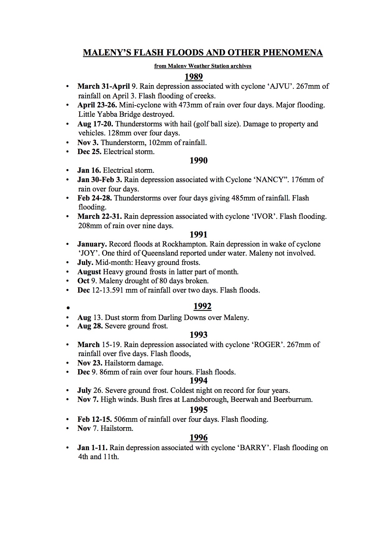
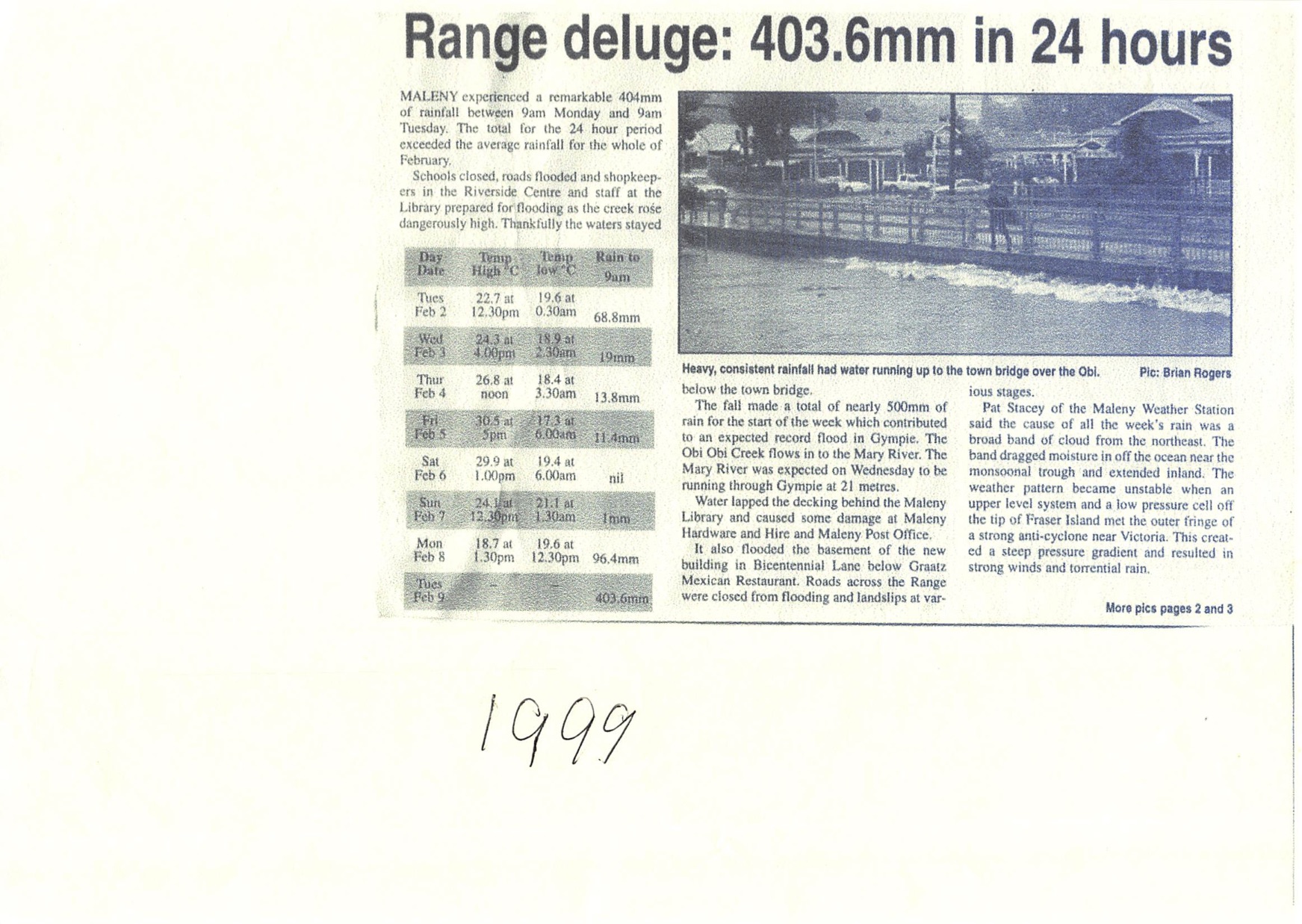
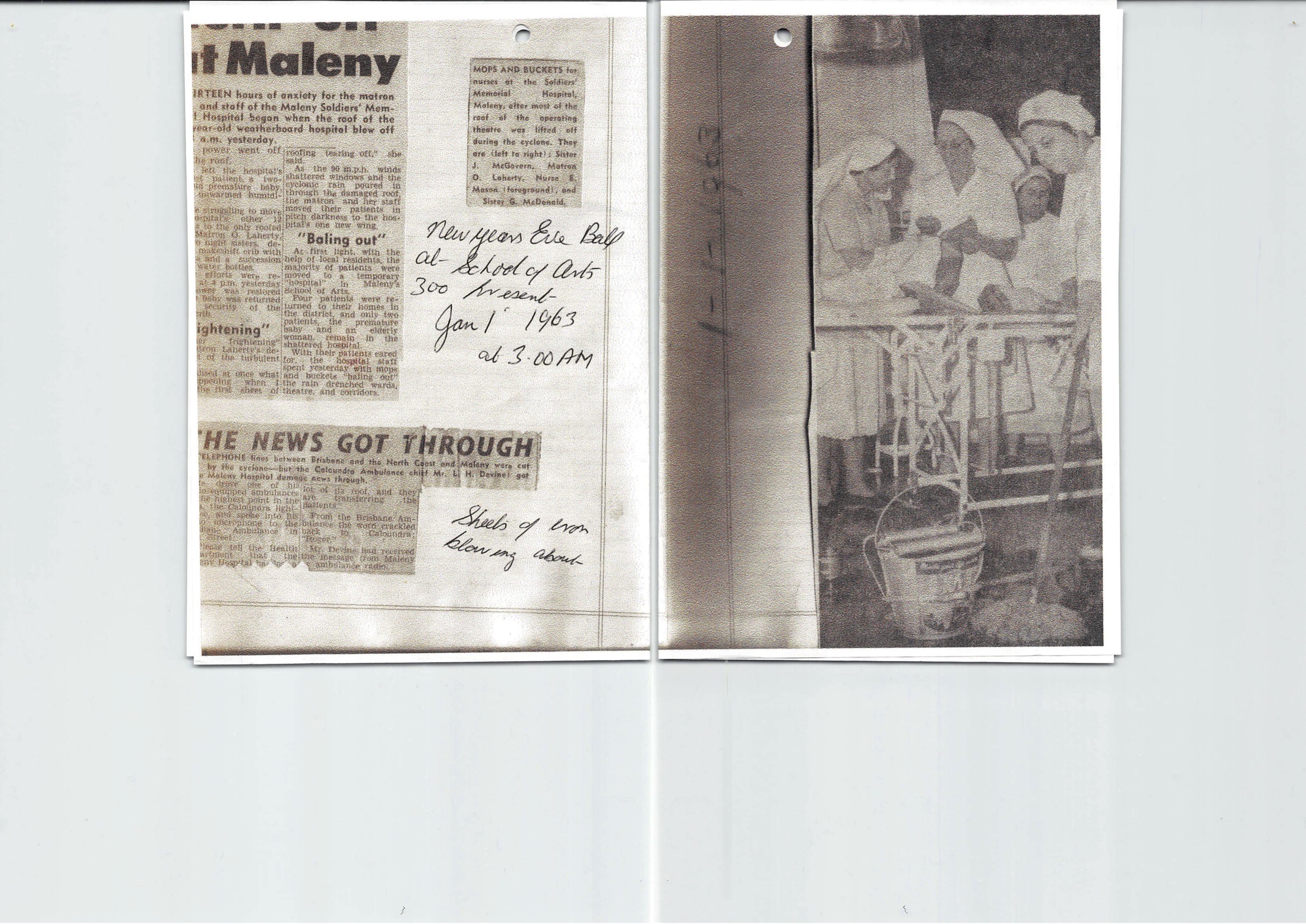
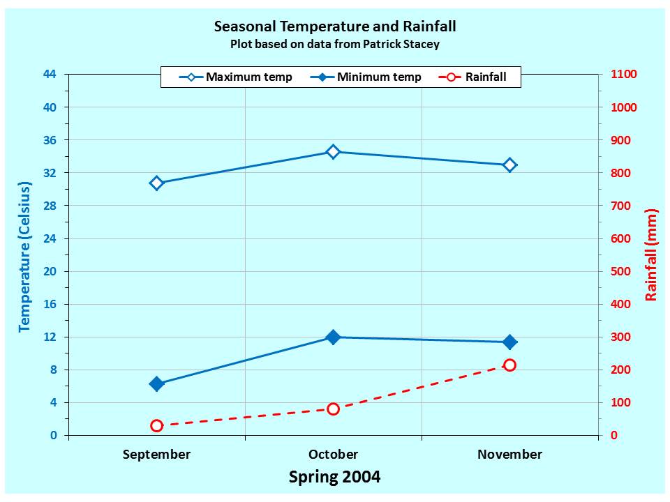
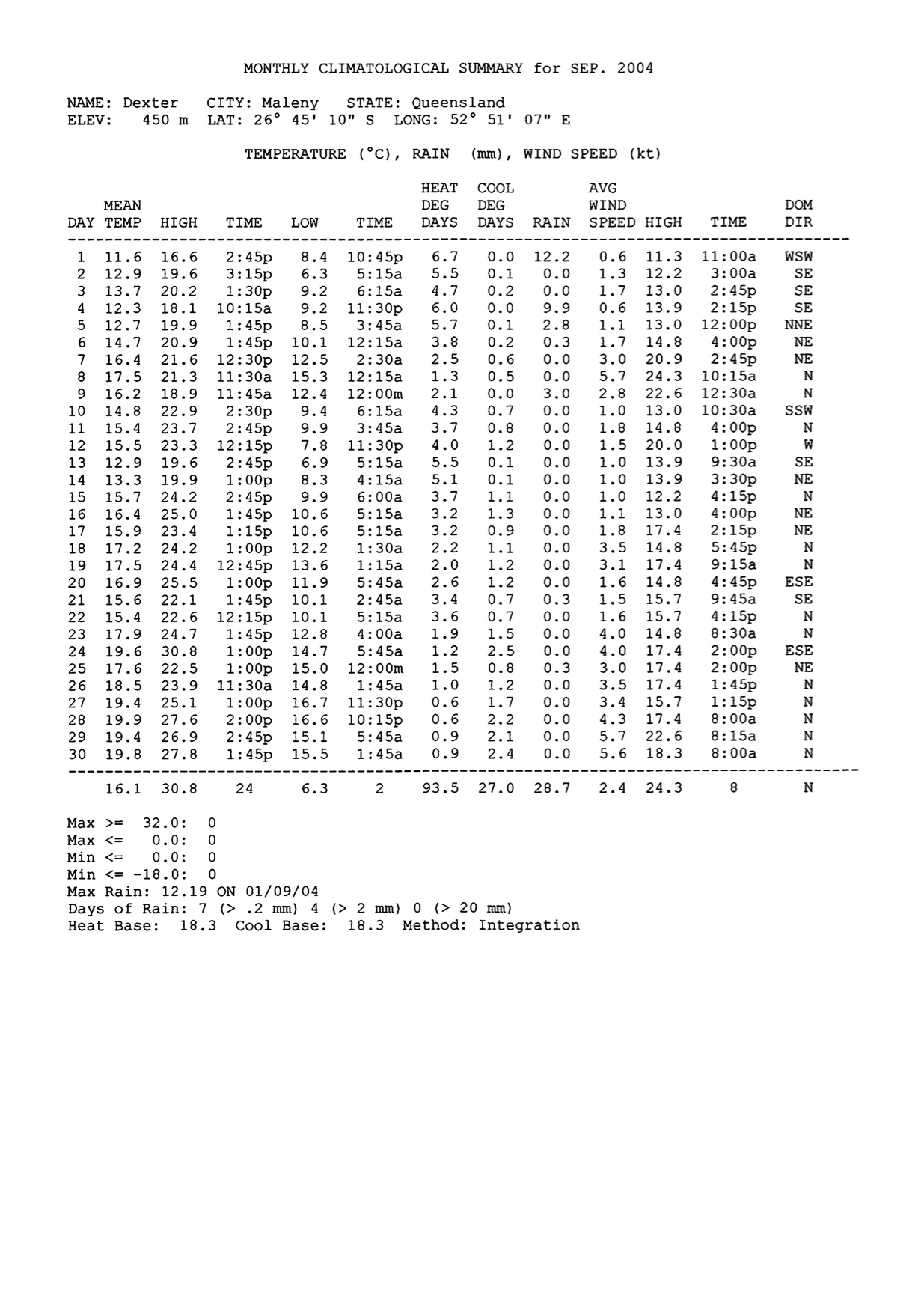
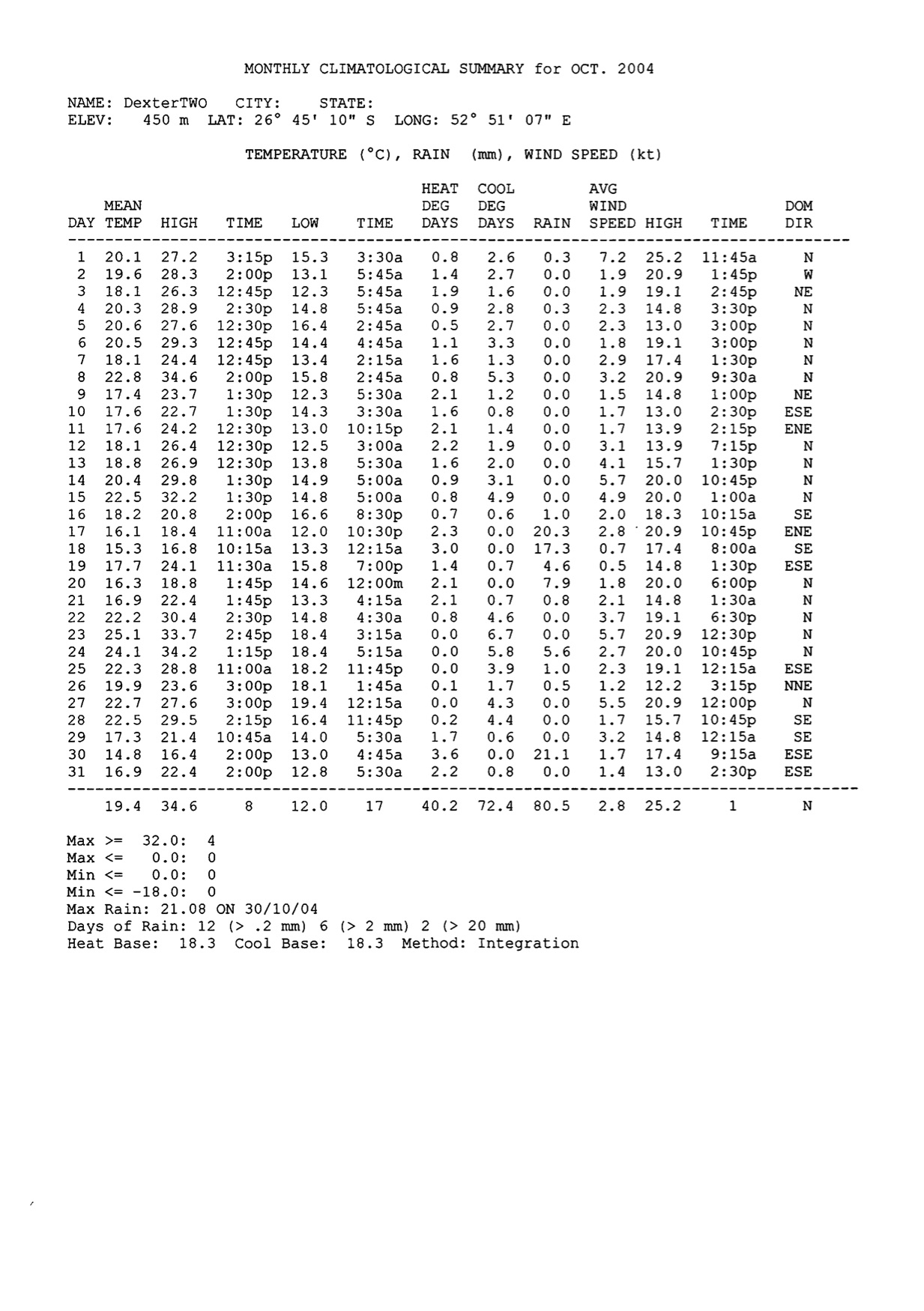
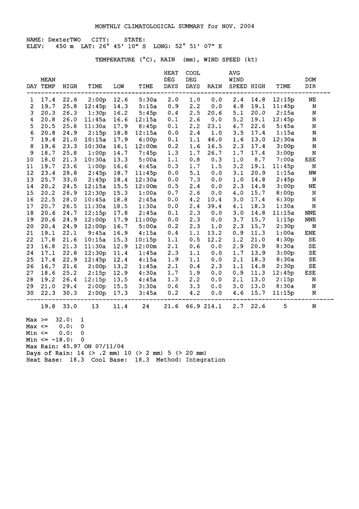
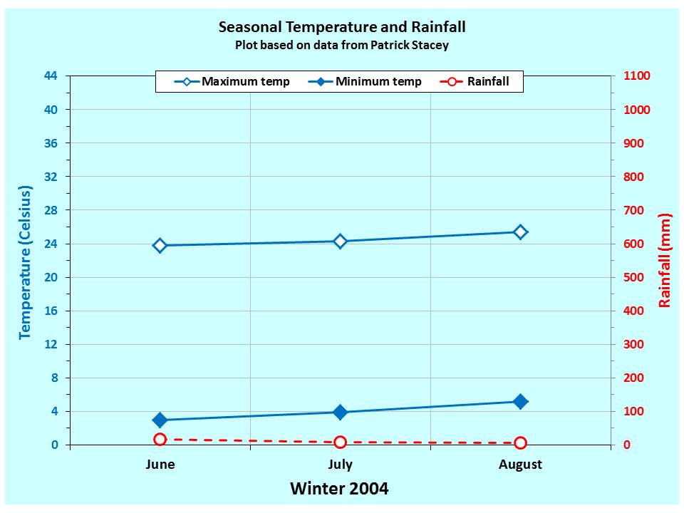
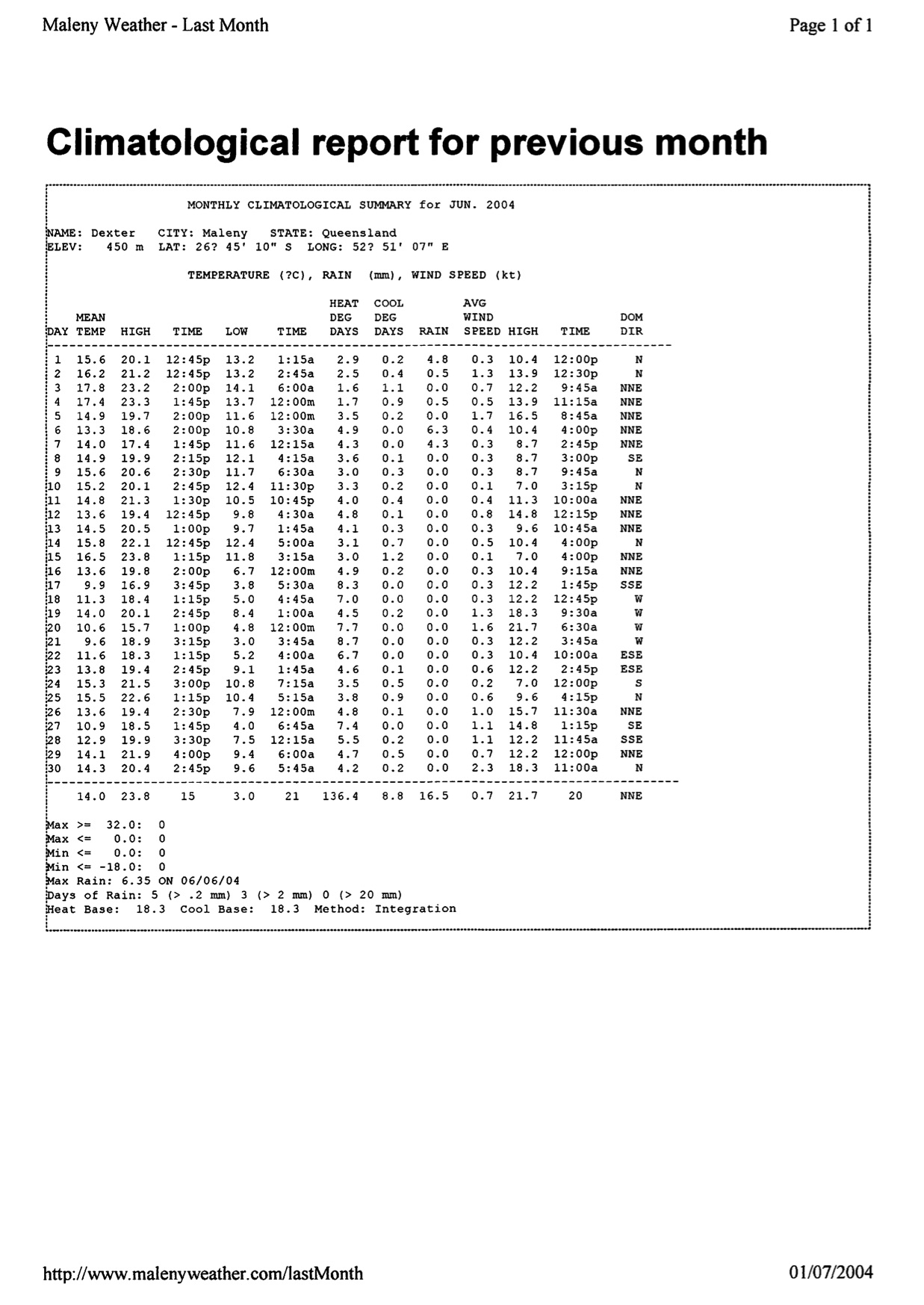
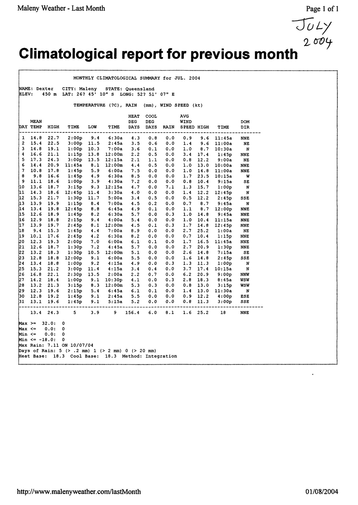
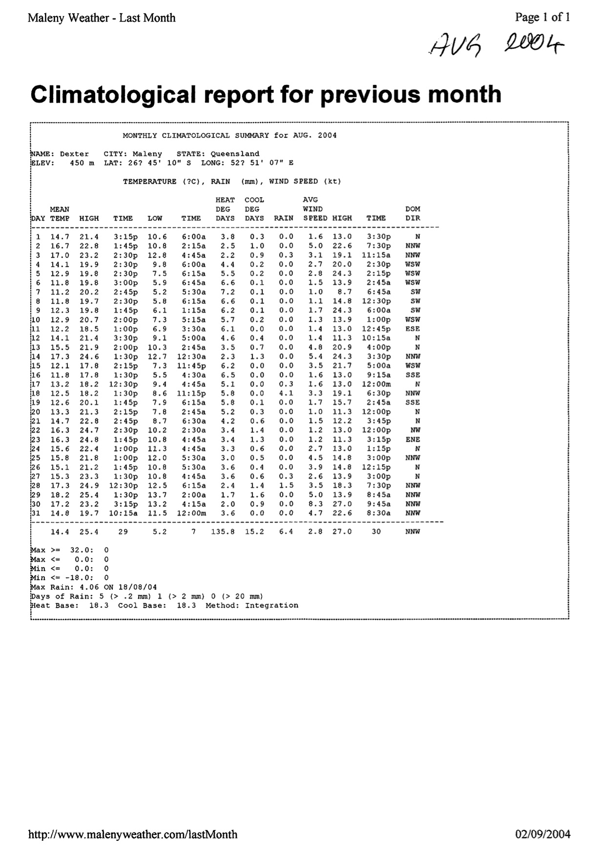
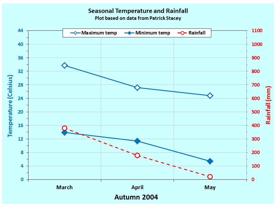
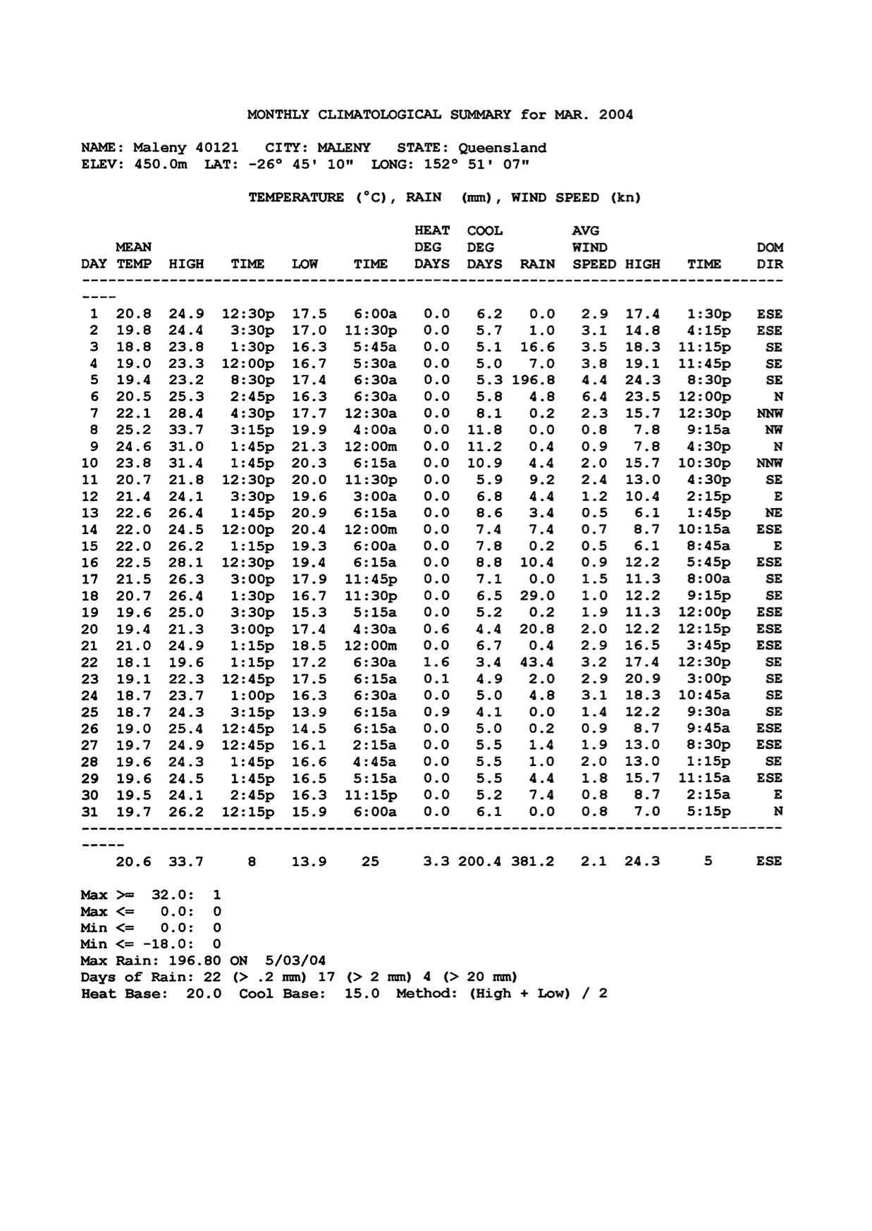
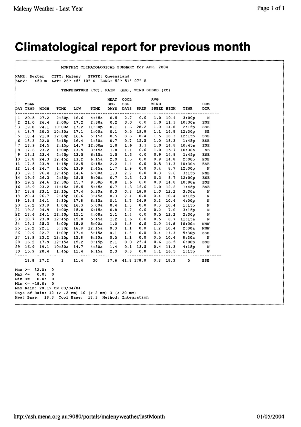
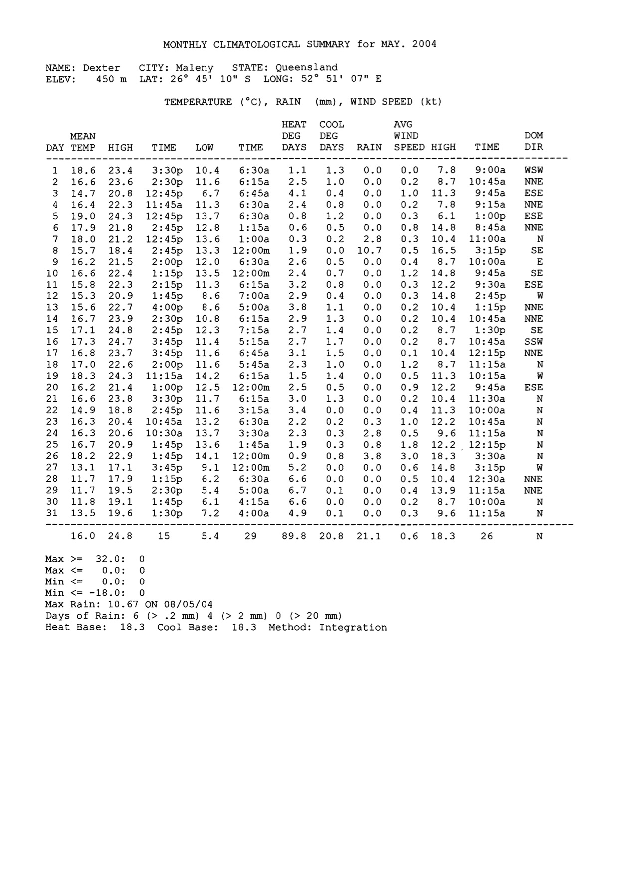
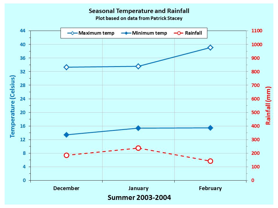

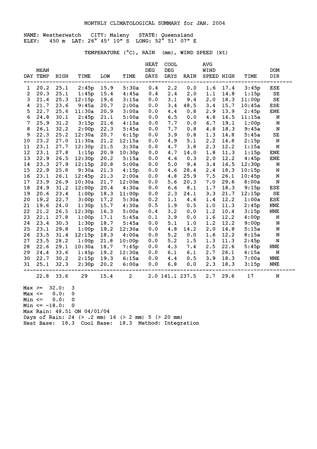
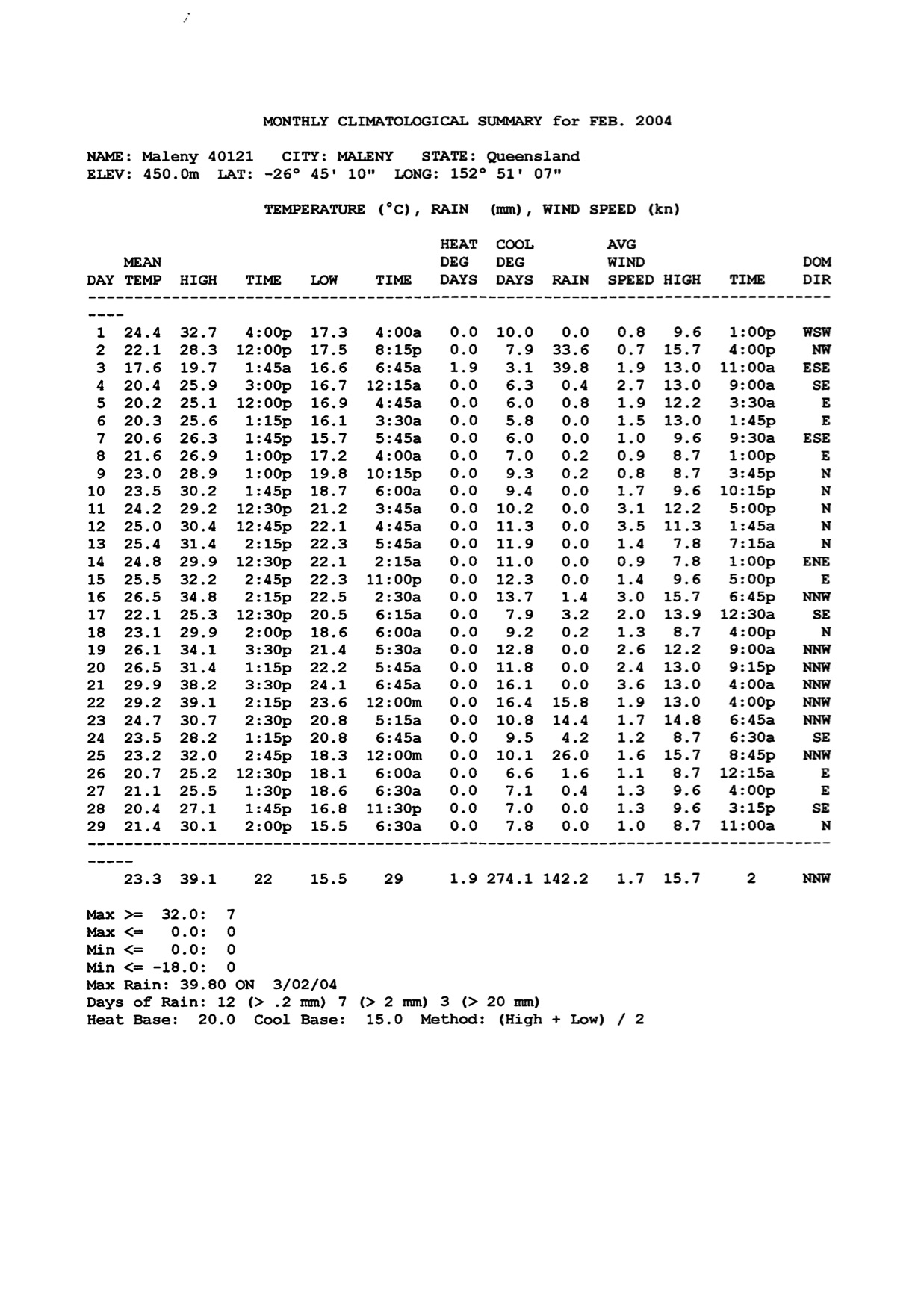
Sir William Thomson, Lord Kelvin (1824 – 1907)
Sir William Thomson, Lord Kelvin (1824 – 1907)
Kelvin was a Scottish mathematician and physicist who developed the Kelvin scale of temperature measurement.
William Thomson was born on 26 June 1824 in Belfast. He was taught by his father, a professor of mathematics. In 1832, the family moved to Glasgow where Thomson attended university from the age of 10, subsequently studying at Cambridge and Paris universities. In 1846 he became professor of natural philosophy in Glasgow, a post he would hold for more than 50 years.
In Glasgow, Thomson created the first physics laboratory in Britain. He was a pioneer in many different fields, particularly electromagnetism and thermodynamics. Together with Faraday, he was responsible for the introduction of the concept of an electromagnetic field. In thermodynamics, Thomson assimilated and developed the work of the pioneers of the subject, Nicolas Carnot and James Joule. One of the most important results of his work was his idea of an absolute zero of temperature – the scale based on this is named after him.
Throughout his work Thomson’s overriding goal was the practical utilisation of science. He achieved fame through his work on submarine telegraphy, a major practical problem of the day. Kelvin was employed as a scientific adviser in the laying of the Atlantic telegraph cables in 1857-1858 and 1865-1866, for which he was knighted in 1866. His interest in marine issues also inspired him to develop a mariners’ compass and invent a tide machine and depth-measuring equipment. He invented many electrical instruments and his house in Glasgow was the first to be lit by electric light.
Thomson was raised to the peerage with the title of Baron Kelvin of Largs in 1892 (the Kelvin was a small river that flowed near Glasgow University) and was president of the Royal Society from 1890 to 1895. He died on 17 December 1907 in Ayrshire, Scotland and was buried in Westminster Abbey.
Gabriel Fahrenheit
Gabriel Fahrenheit Biography
Born: May 14, 1686
Danzig, Germany
Died: September 16, 1736
The Hague, the Netherlands
German instrument maker and glassblower
The German instrument maker Gabriel Fahrenheit made the first reliable thermometers, and the temperature scale he created is named after him.
Early life
Born in Danzig, Germany, on May 14, 1686, Gabriel Daniel Fahrenheit was one of Daniel and Concordia Schumann Fahrenheit’s five children. His father was a wealthy merchant. Both his parents died on the same day, August 14, 1701, and he was then sent to Amsterdam, the Netherlands, to work for and learn from a shopkeeper. After completing a term of four years there, Fahrenheit became interested in making scientific instruments. Although he lived in Amsterdam most of his life, he traveled widely to observe the work of scientists and makers of instruments in other areas. He spent considerable time in England, where he became a member of the Royal Society (Great Britain’s oldest organization of scientists).
Creation of thermometers
Fahrenheit completed his first two thermometers by 1714. They contained alcohol and agreed exactly in their readings. The scale that was to bear Fahrenheit’s name had not yet been made standard, and many different scales were tried before he settled on one. He soon decided to replace the alcohol with mercury and completed a series of investigations based on the work of Danish astronomer Olaus Roemer. In these investigations he determined the boiling point of water and other liquids and studied the expansion (increase in volume) properties of mercury. These experiments led to the discovery that the boiling point of water varies with changes in the pressure of the atmosphere. Fahrenheit also discovered the method of supercooling water—that is, cooling water to below its normal freezing point without it becoming ice.
Taking all of these factors into consideration, Fahrenheit began to doubt the reliability of the freezing and boiling points of water. He finally settled on a temperature scale ranging from 0 to 212. In 1724, announcing his method of making thermometers in the Philosophical Transactions of the Royal Society, he described how he used the temperatures of the human body and of a mixture of water, ice, and sea salt to be his high and low measuring points. He set 0 as the temperature of the mixture, 32 as the temperature of water and ice, and 212, a point selected by chance, as the approximate boiling point of water.
Success and new developments
Fahrenheit’s thermometers were very popular. He used mercury successfully because of his method of cleaning it, and he introduced the use of cylinder- shaped bulbs instead of sphere-shaped ones. His detailed process of making thermometers, however, was not made public for some eighteen years, since he wanted to keep his methods a secret. Among the other instruments he created were a constant-weight hydrometer (an instrument to measure the gravity and strength of a liquid), and a “thermobarometer” for estimating barometric pressure (the pressure of the atmosphere) by determining the boiling point of water.
On September 16, 1736, at fifty years old, Fahrenheit died in the Netherlands. He was buried in the city of The Hague. Fahrenheit never married and continued to be active up to his death. Just before he died, he applied for a patent on a machine that would pump water out of polders (drained land in the Netherlands that lies below sea level).

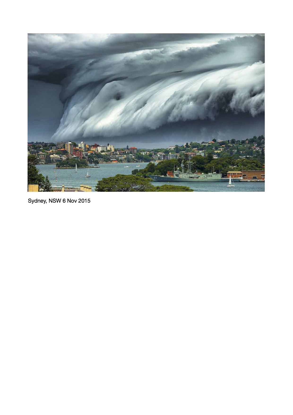
Lenticular Cloud – Mt Fuji
Lenticular Cloud Formation over Mount Fuji.
This is a classic lenticular cloud formation from scalar waves emanating from the mountain. Mountains high in certain minerals such as basalt that contain superconducting monatomic elements (ORMUS), create the vortex-shaped waves which will slice up clouds into disks. The great pyramids mimic this, they are essentially manmade high ORMUS mountains. Google “lenticular clouds” and you’ll see this on other sacred mountains.
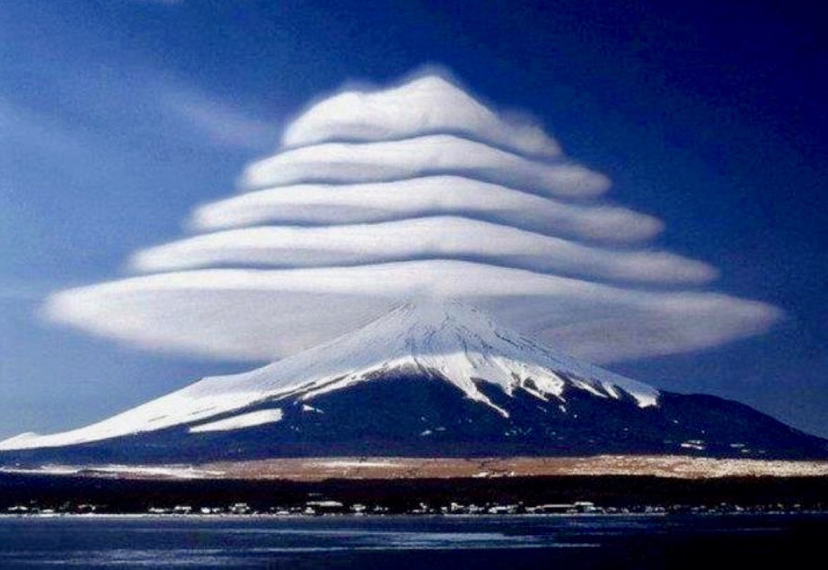
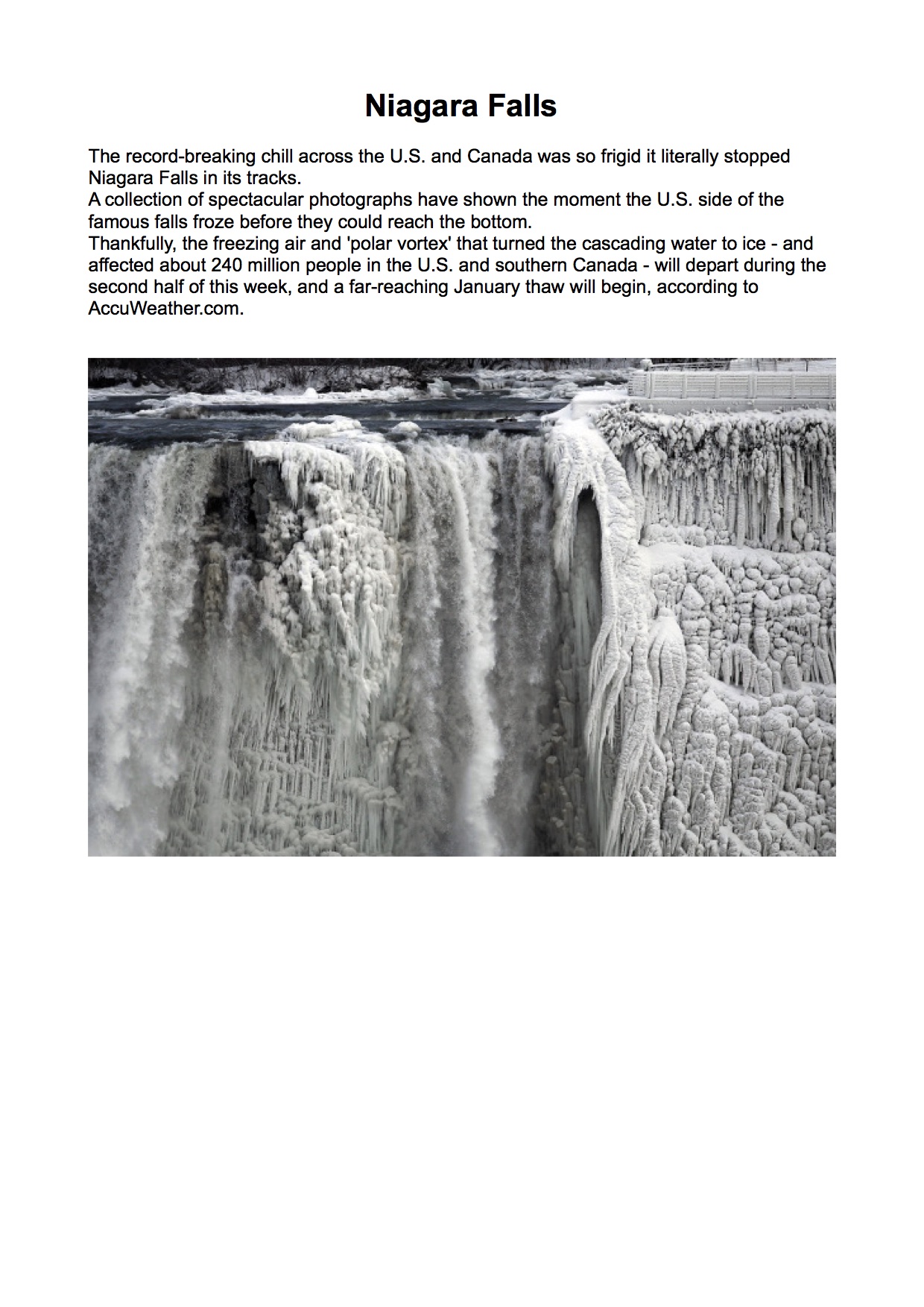
Storm cells over Maleny
Sunday 6th July 2017
In the late afternoon storm cells came in from the west and moved across Maleny. During this one and a half hour event, the Maleny Weather Station recorded some light hail and 3mm rain. Fourteen cloud to ground lightning strikes were recorded ranging from six to twenty Kms away from the Maleny Weather Station.
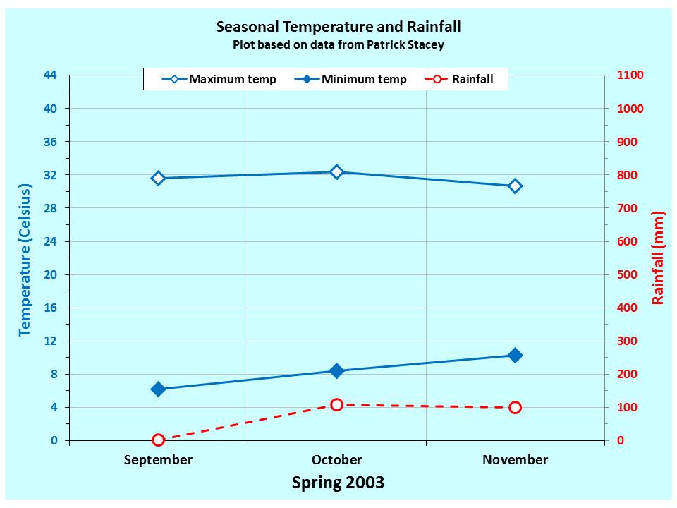
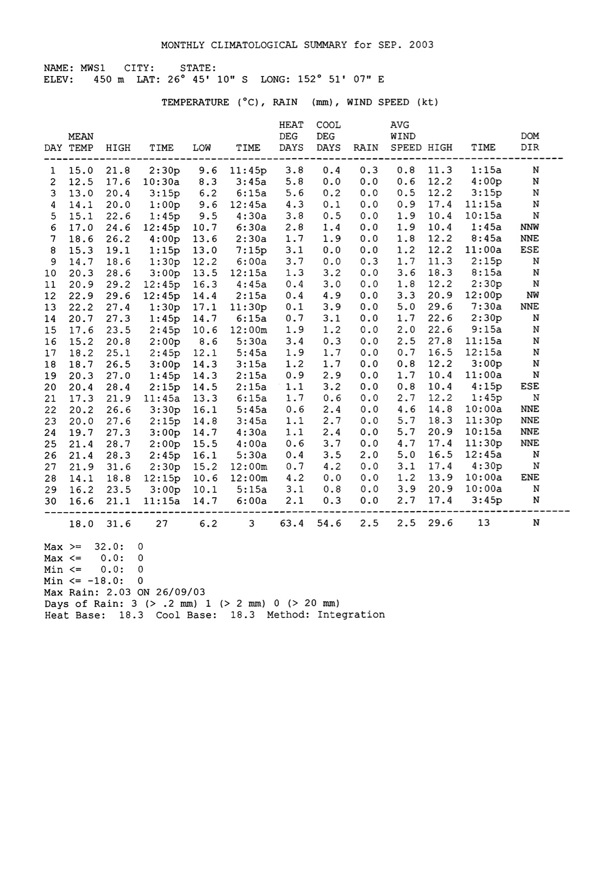

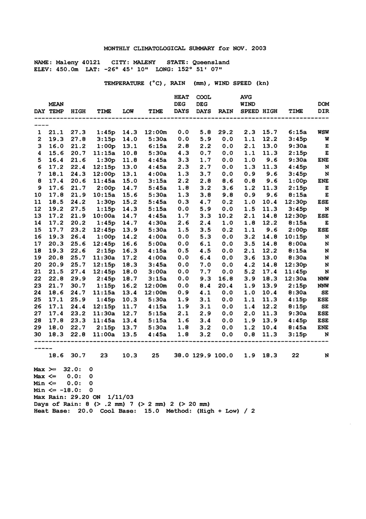
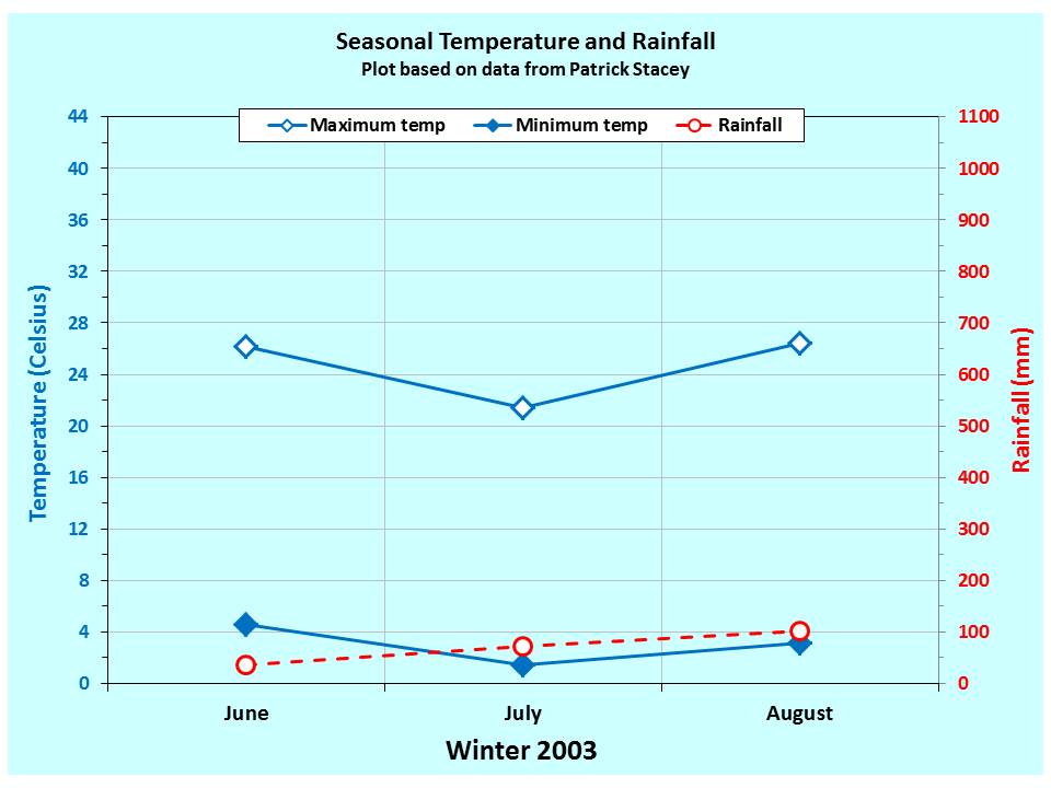
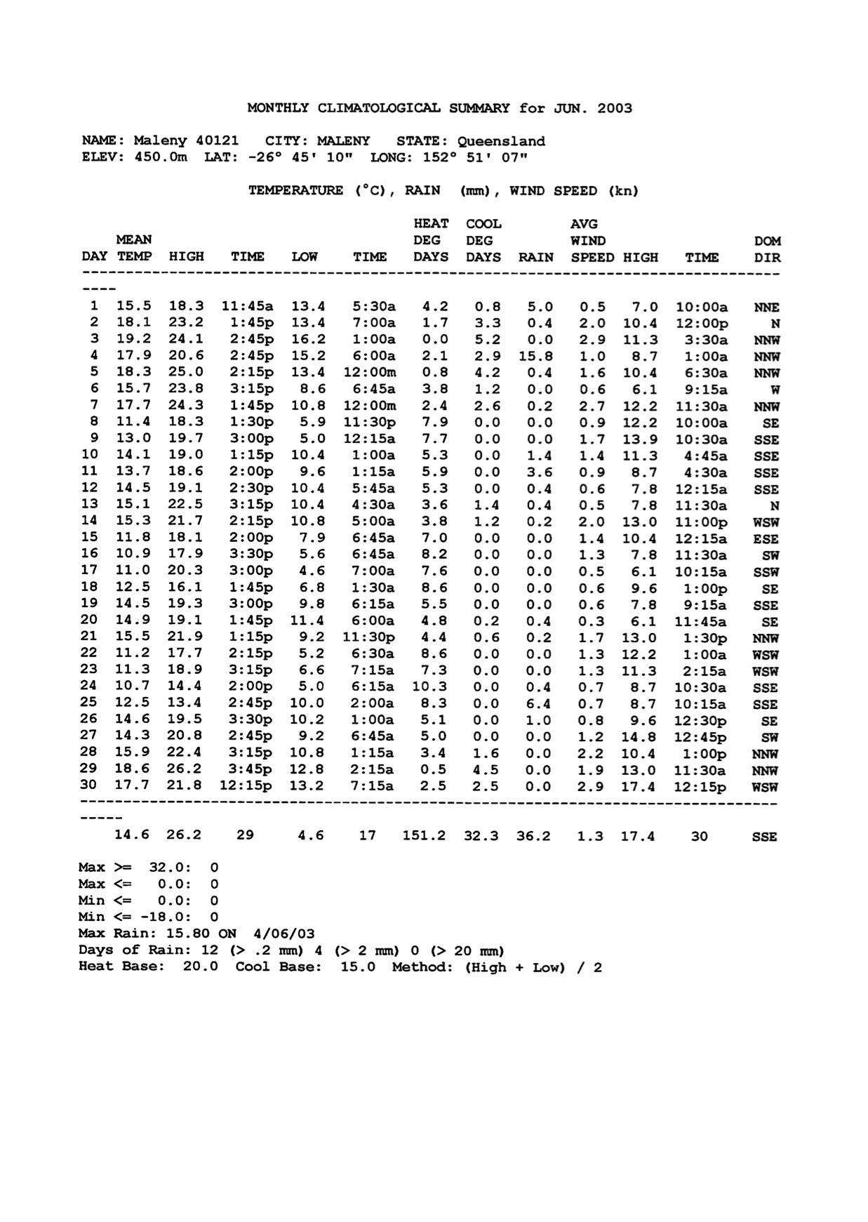
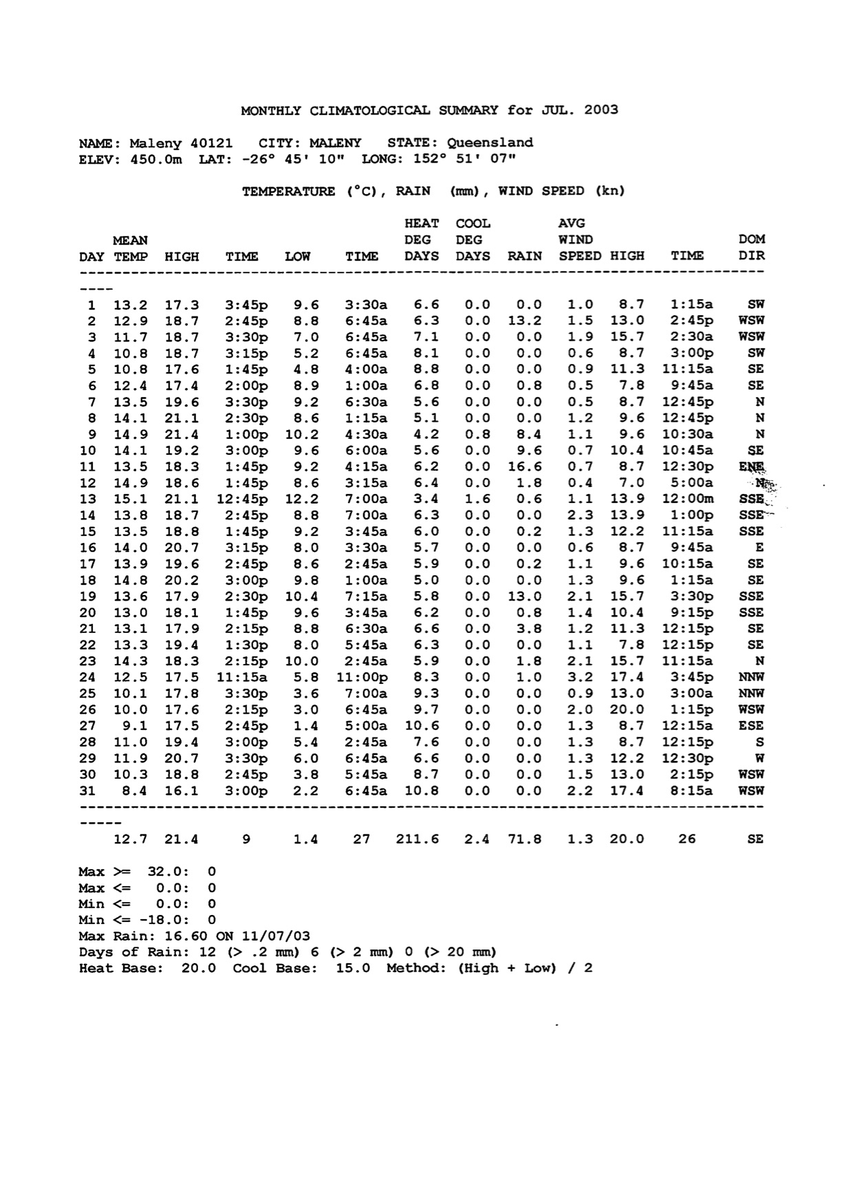
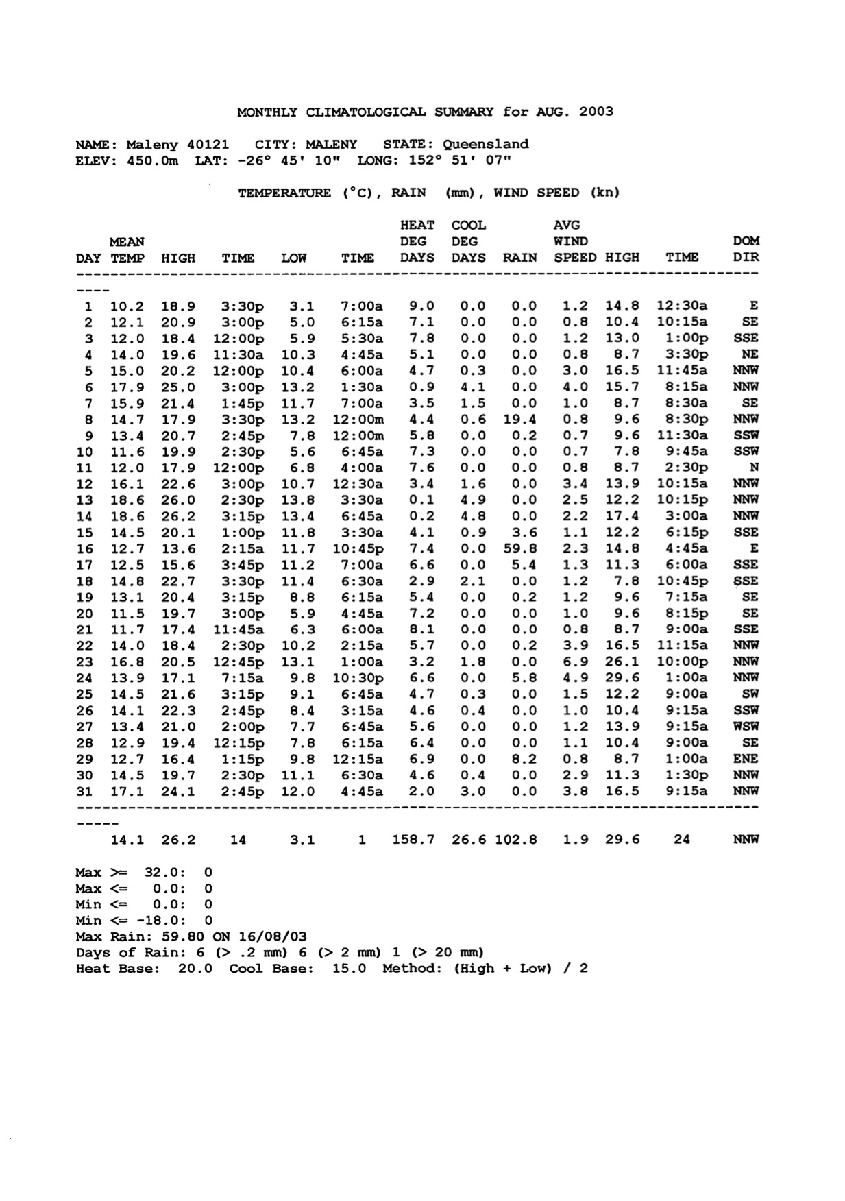
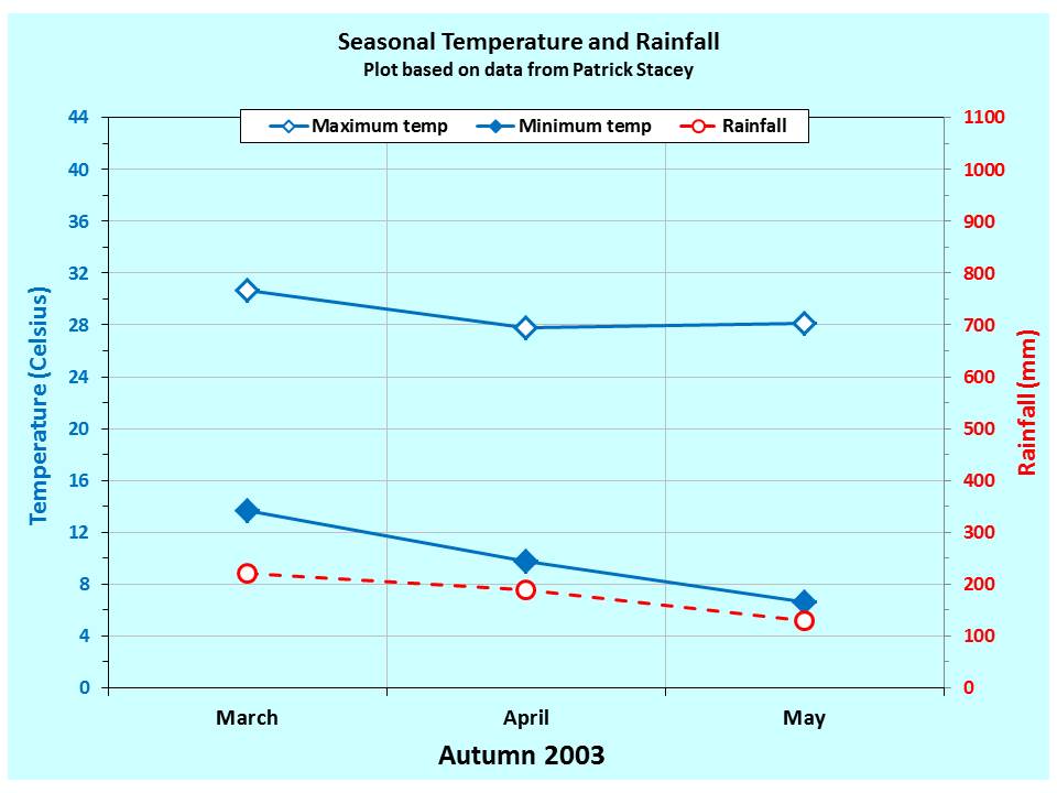
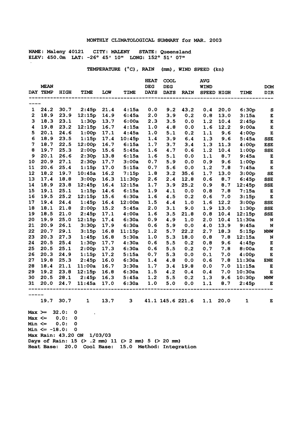
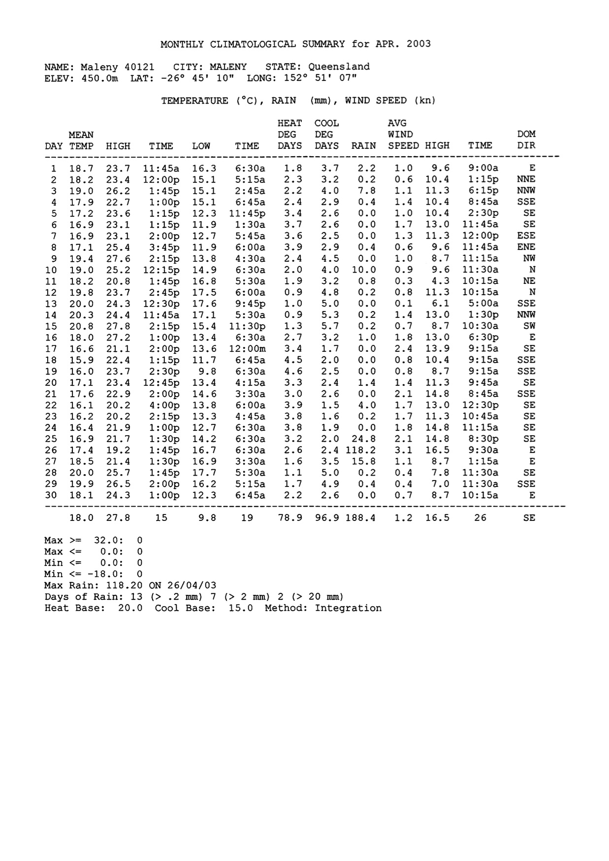
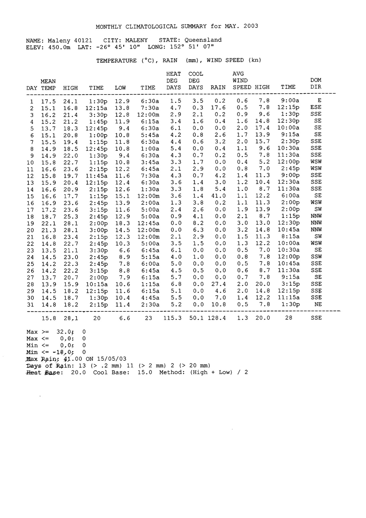

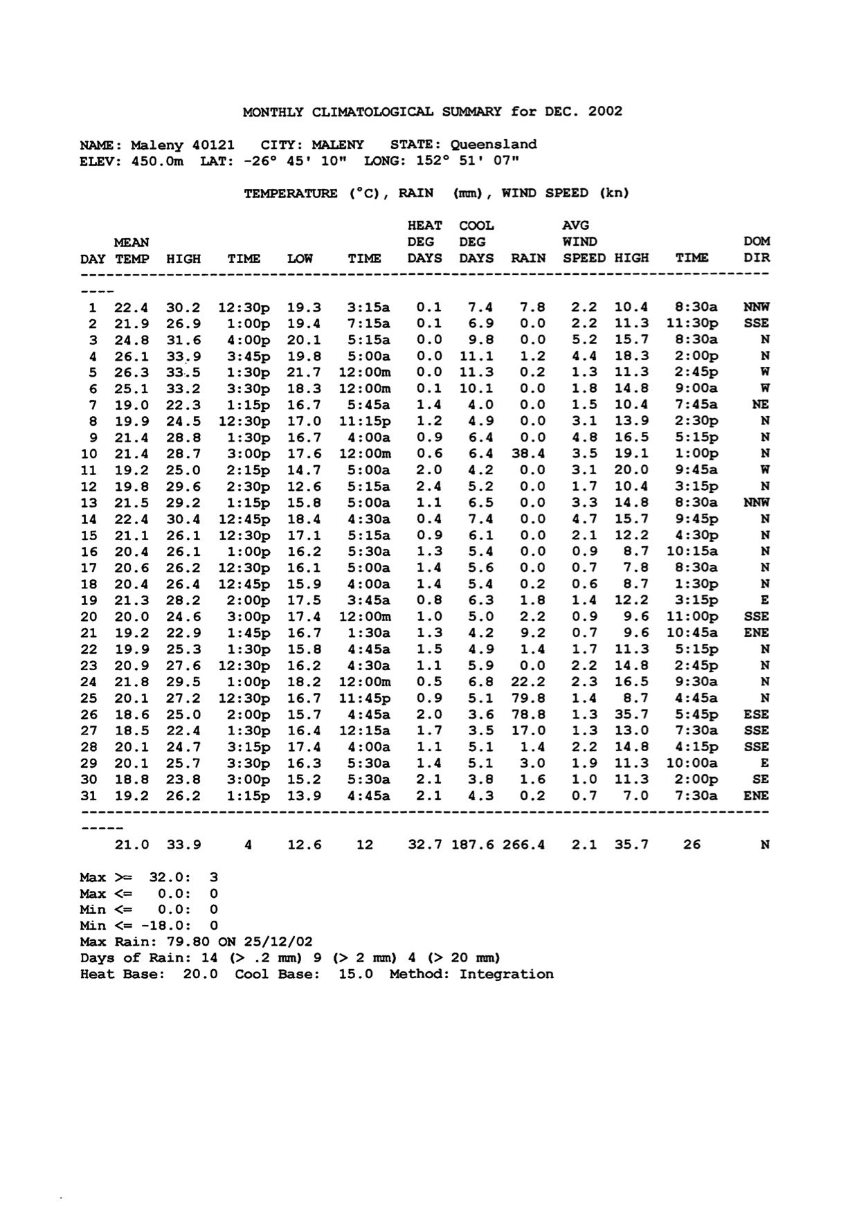
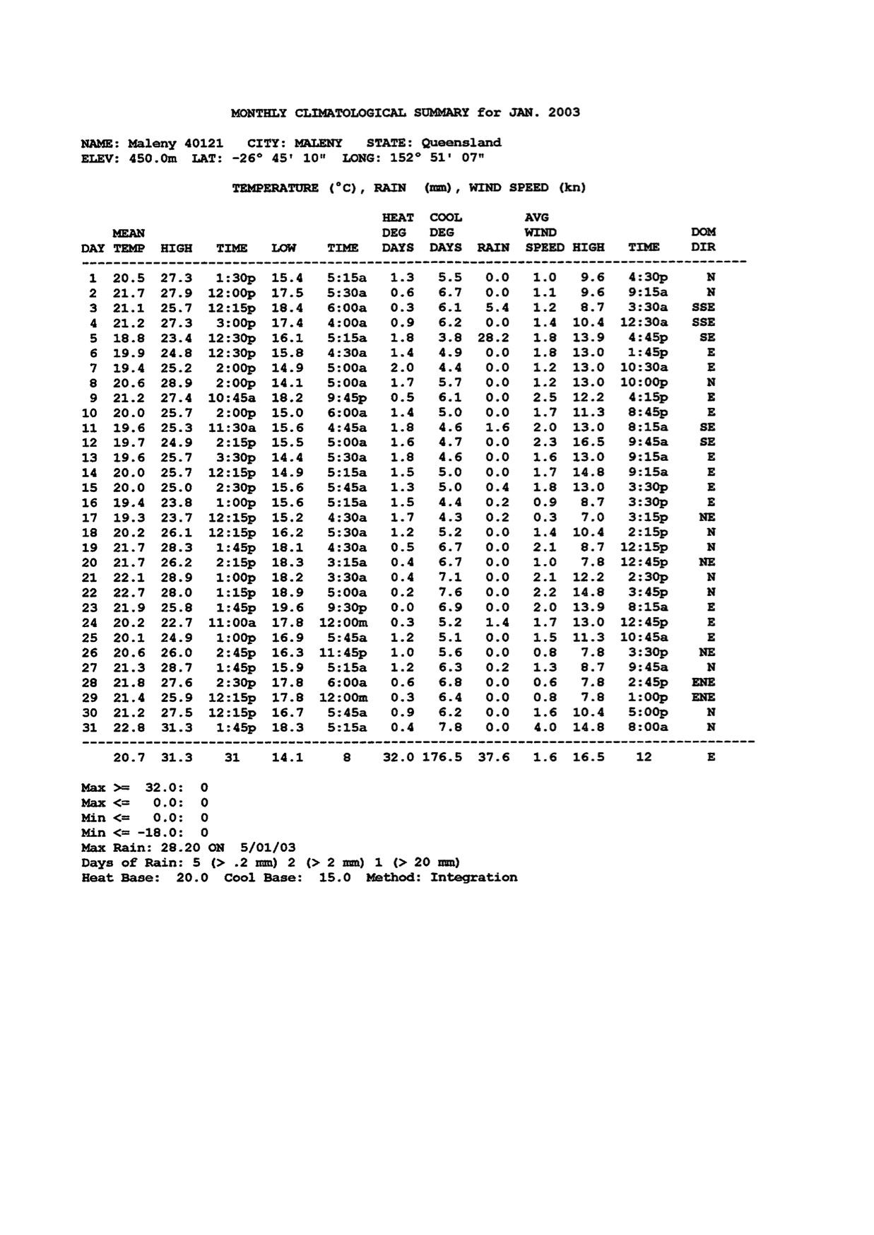


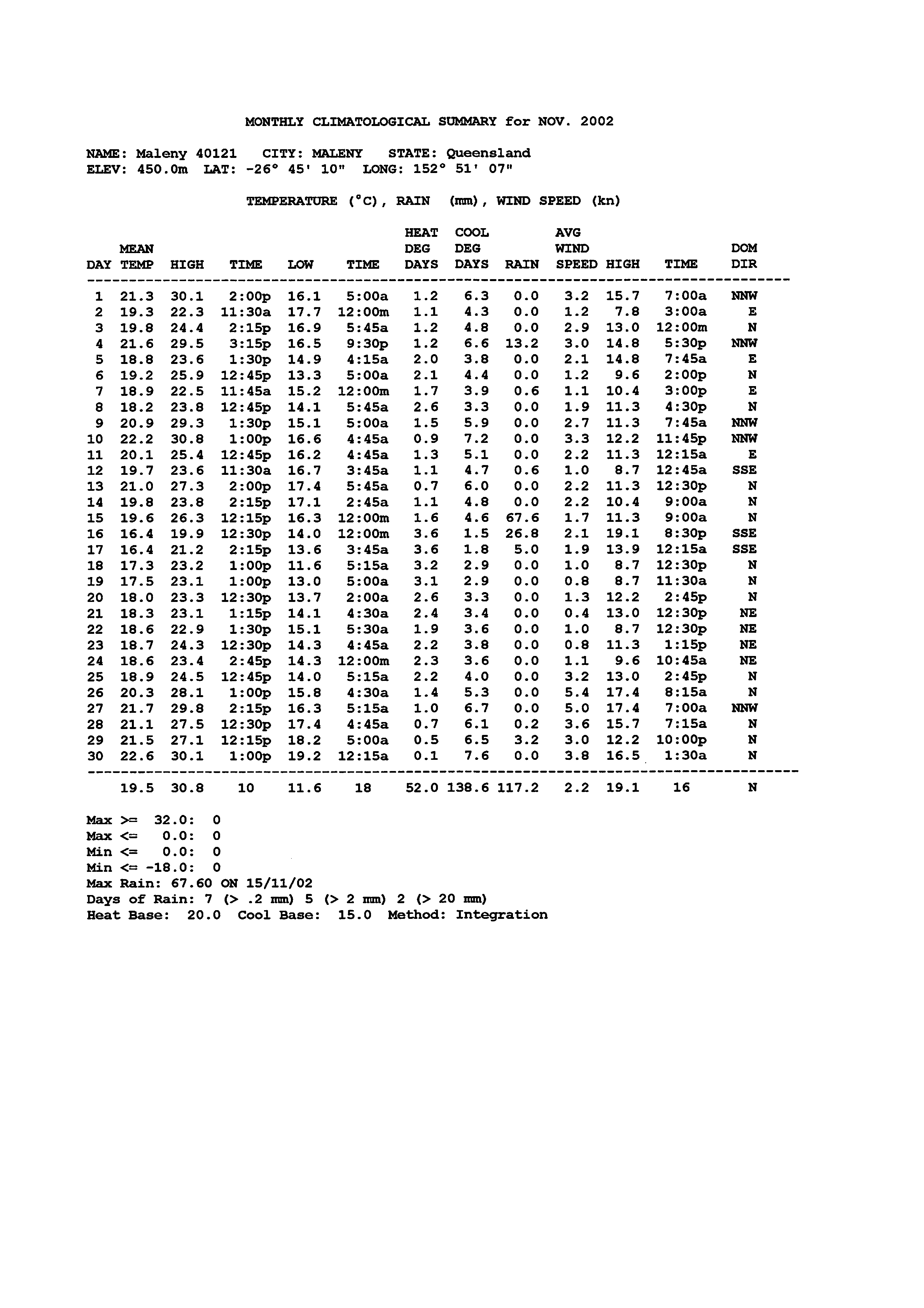
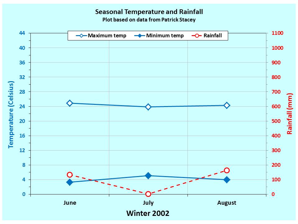
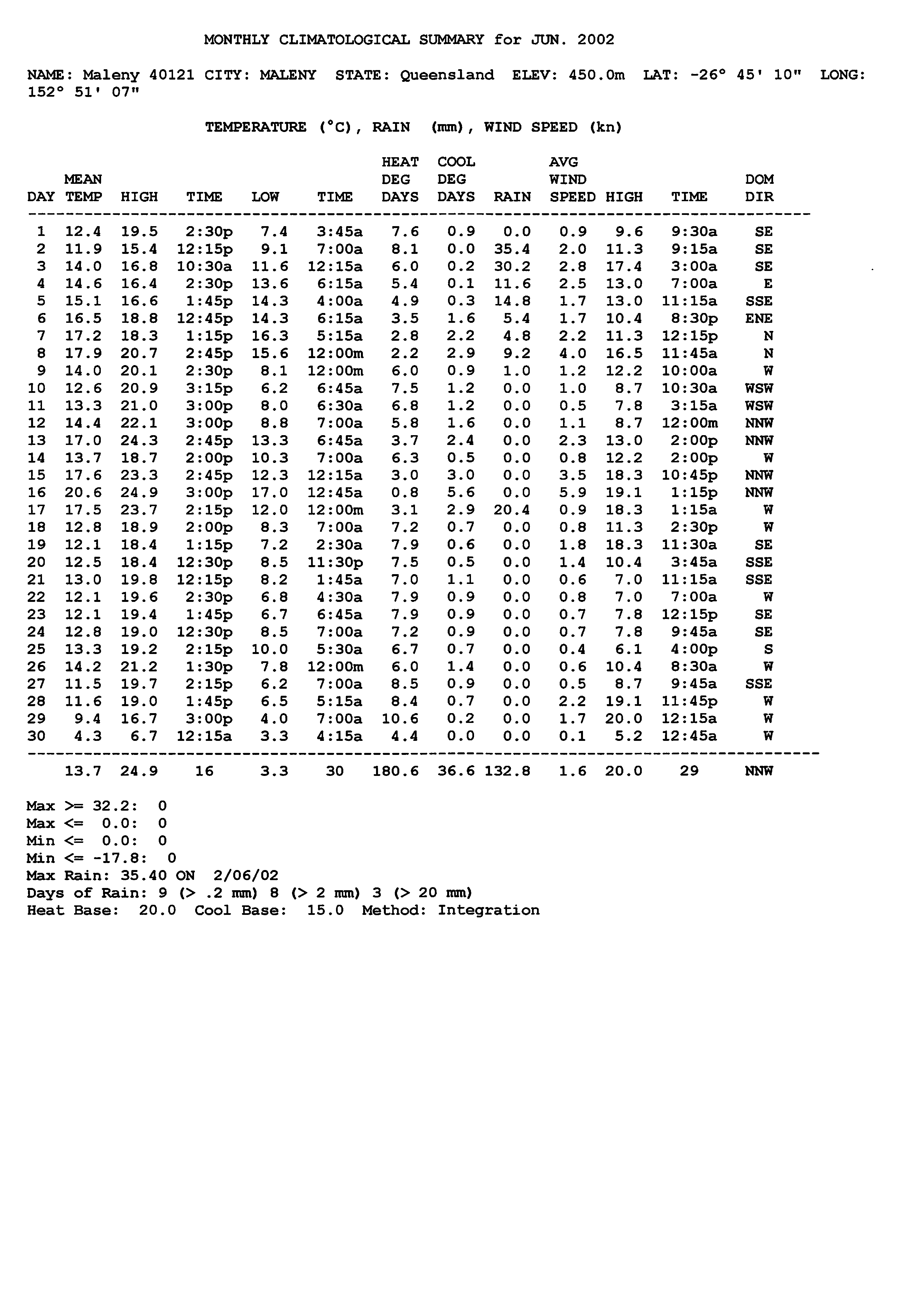
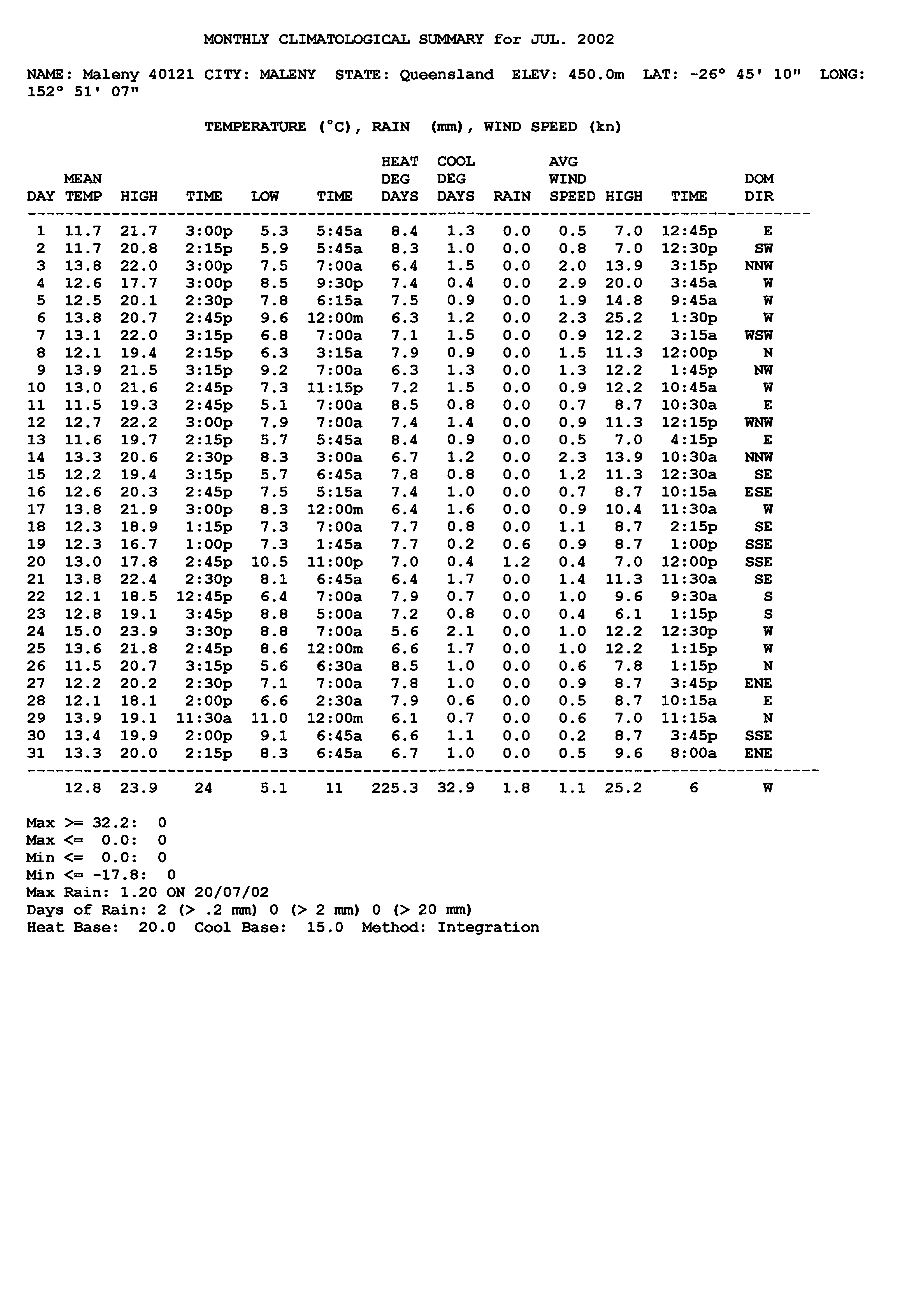
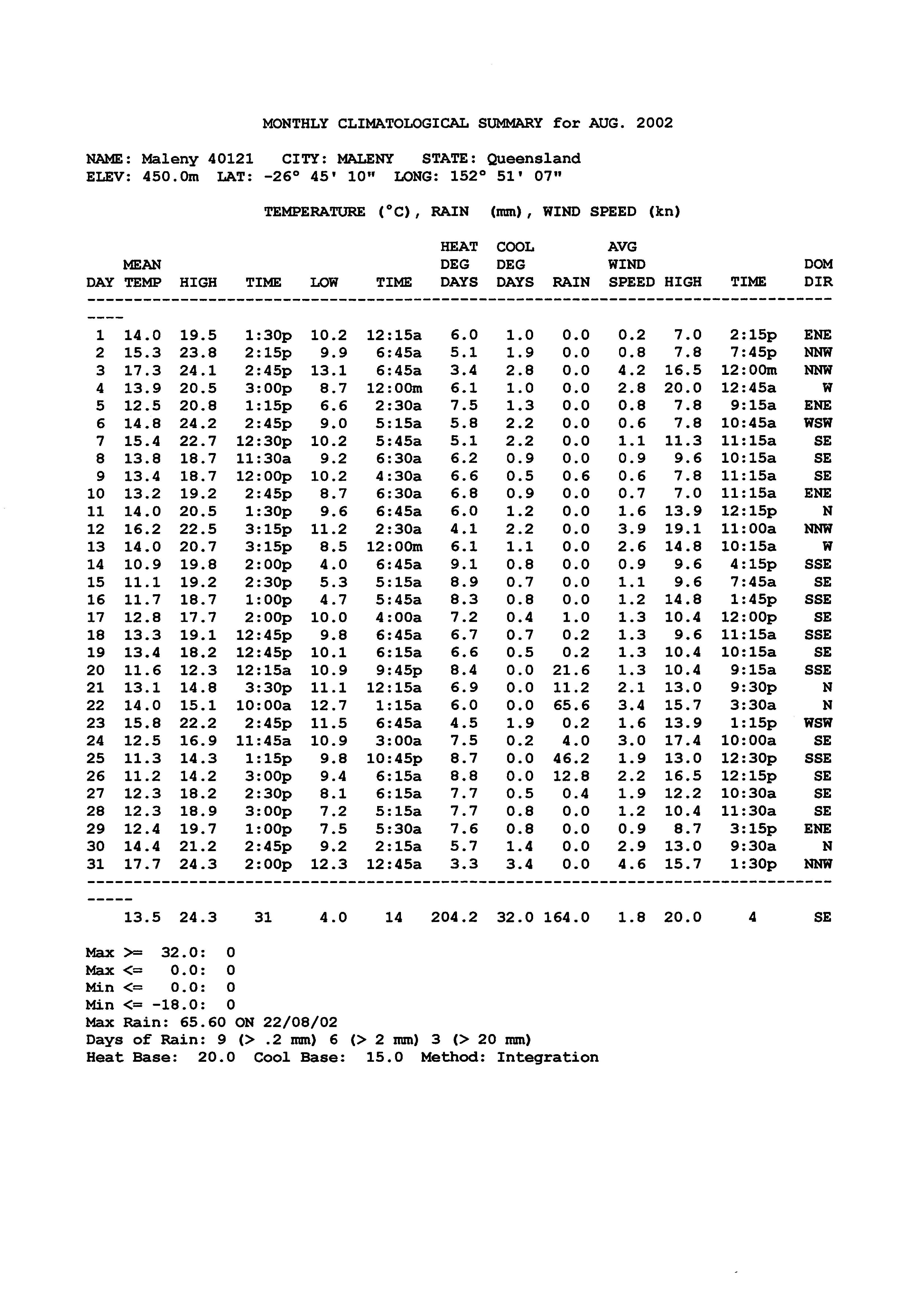
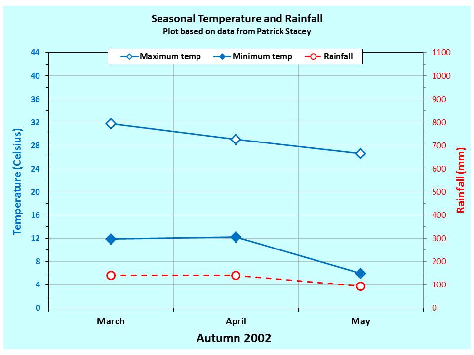
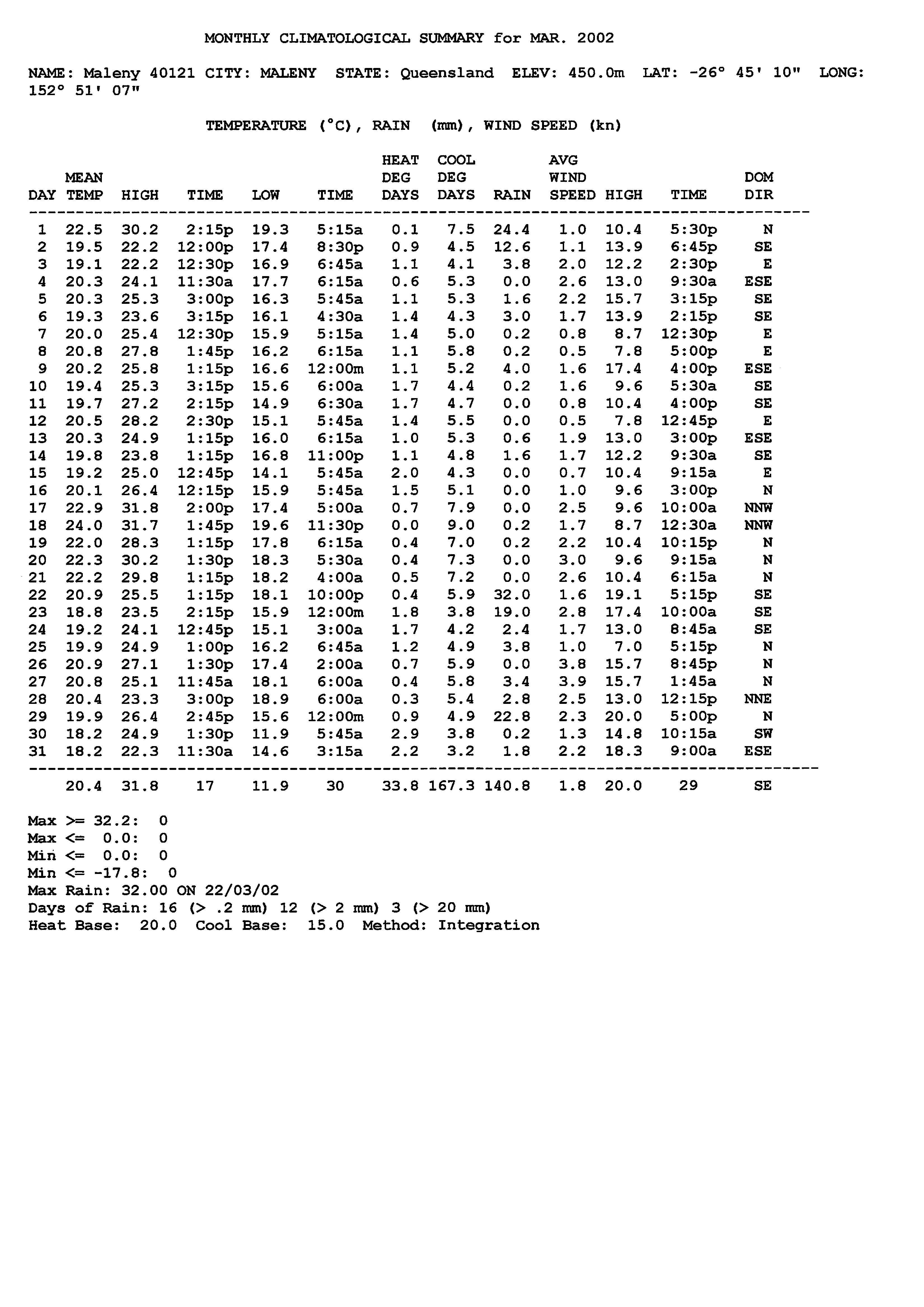

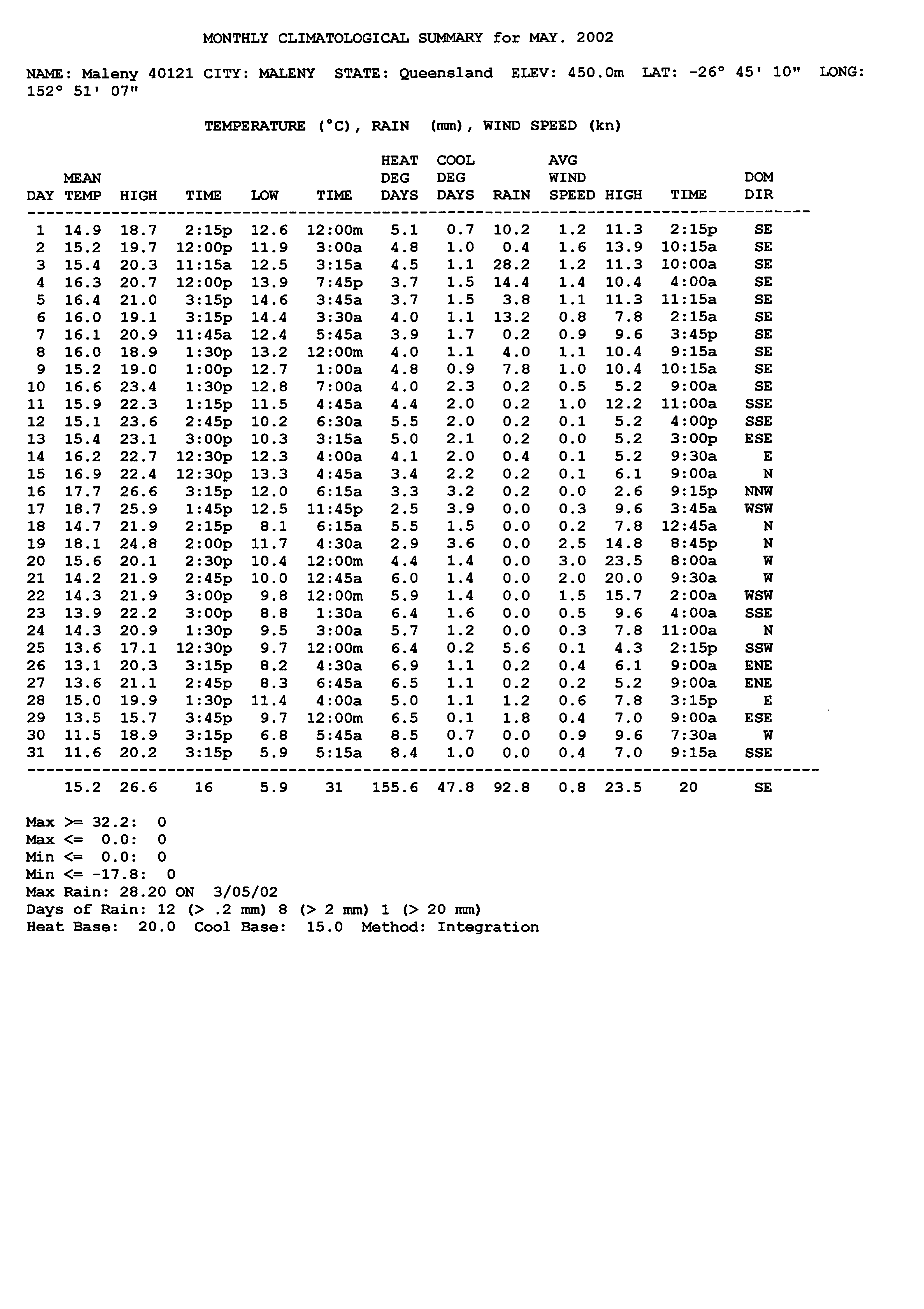
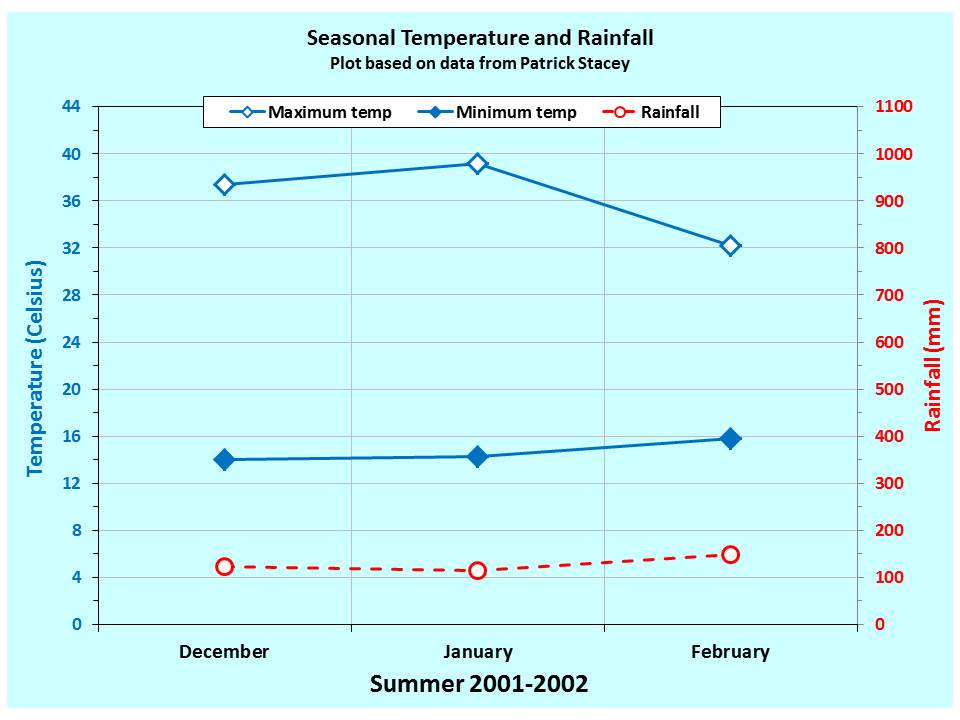


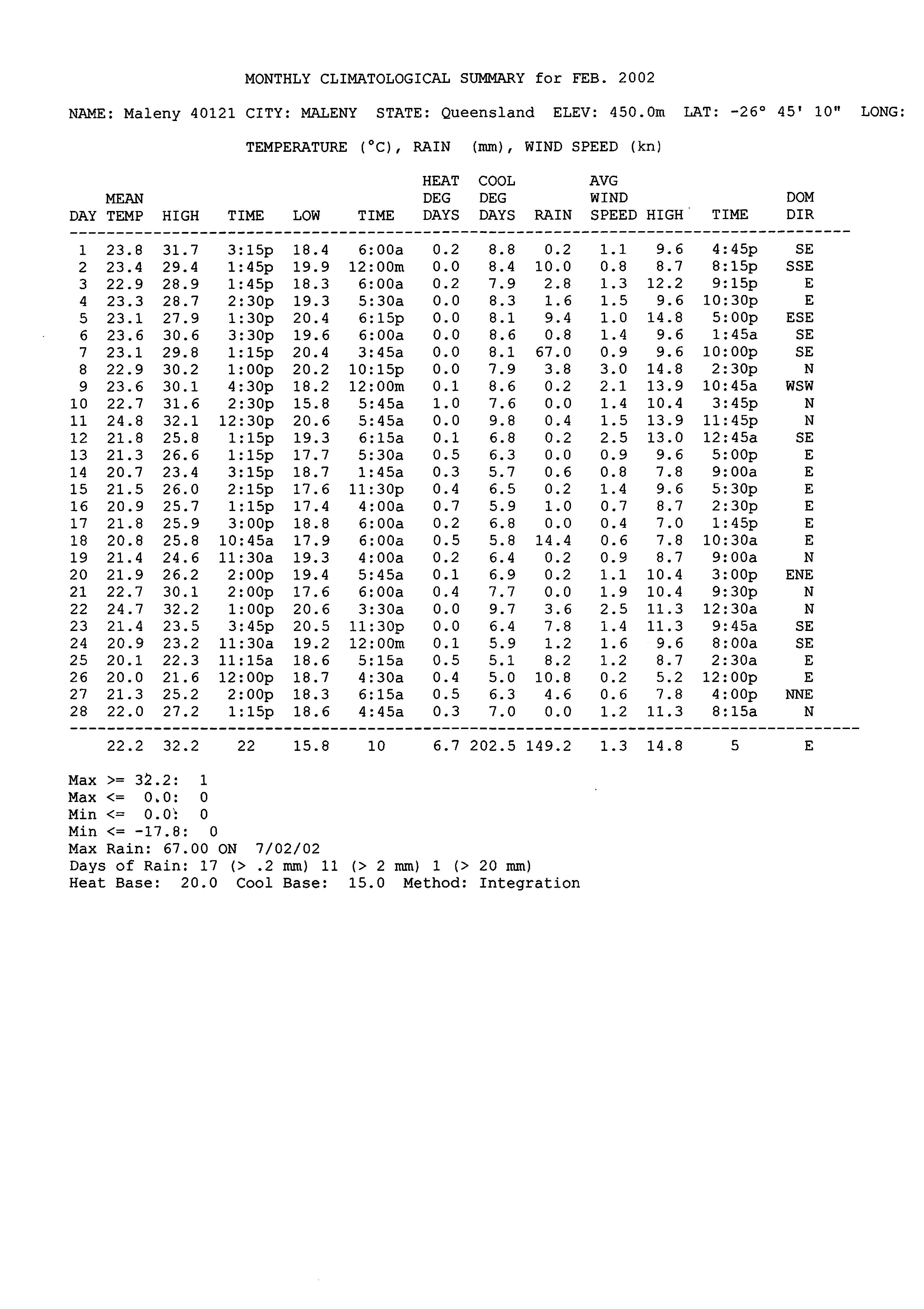


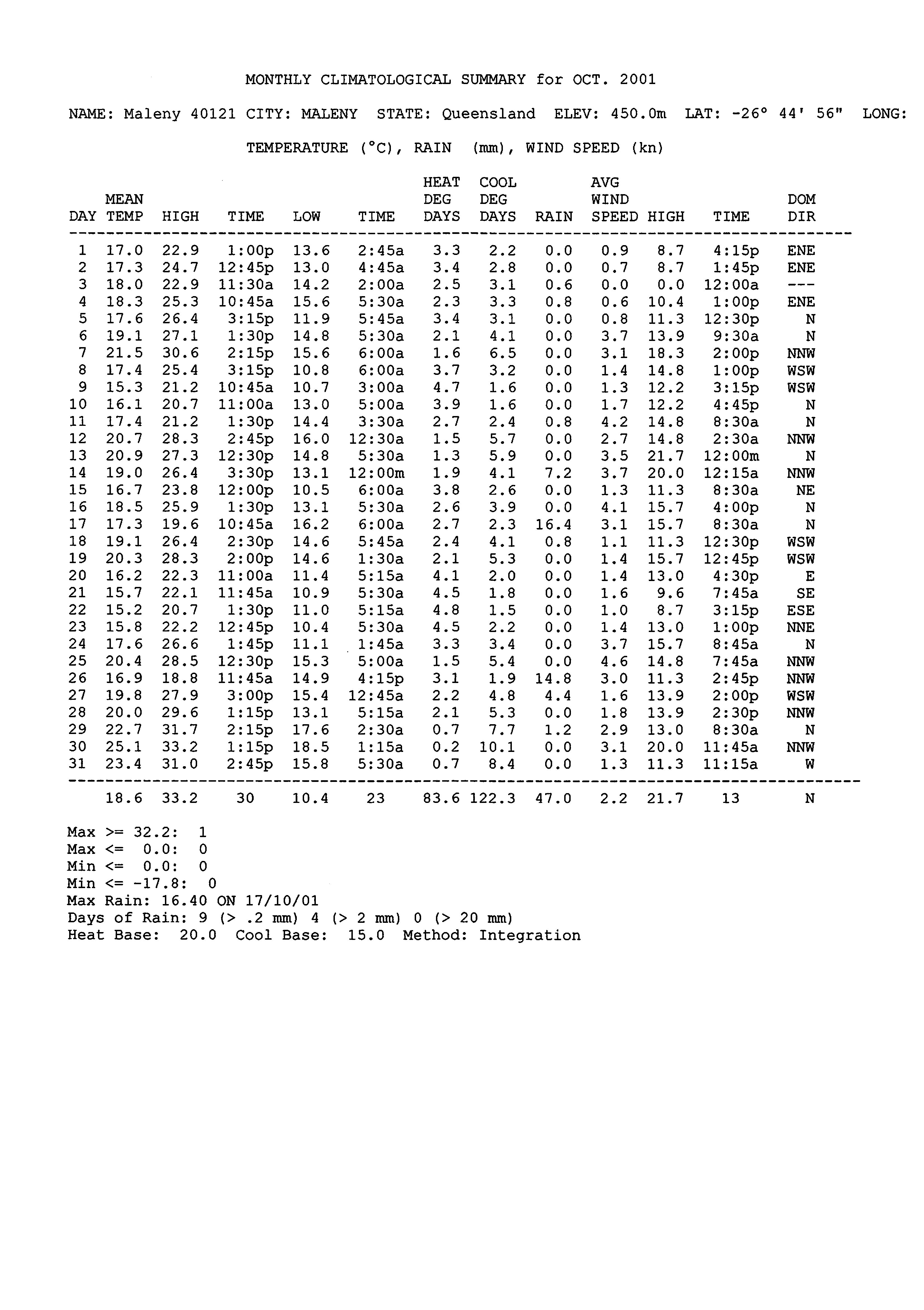

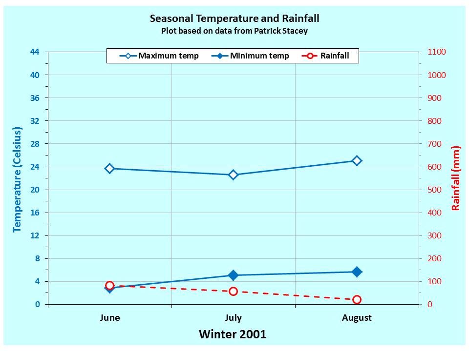


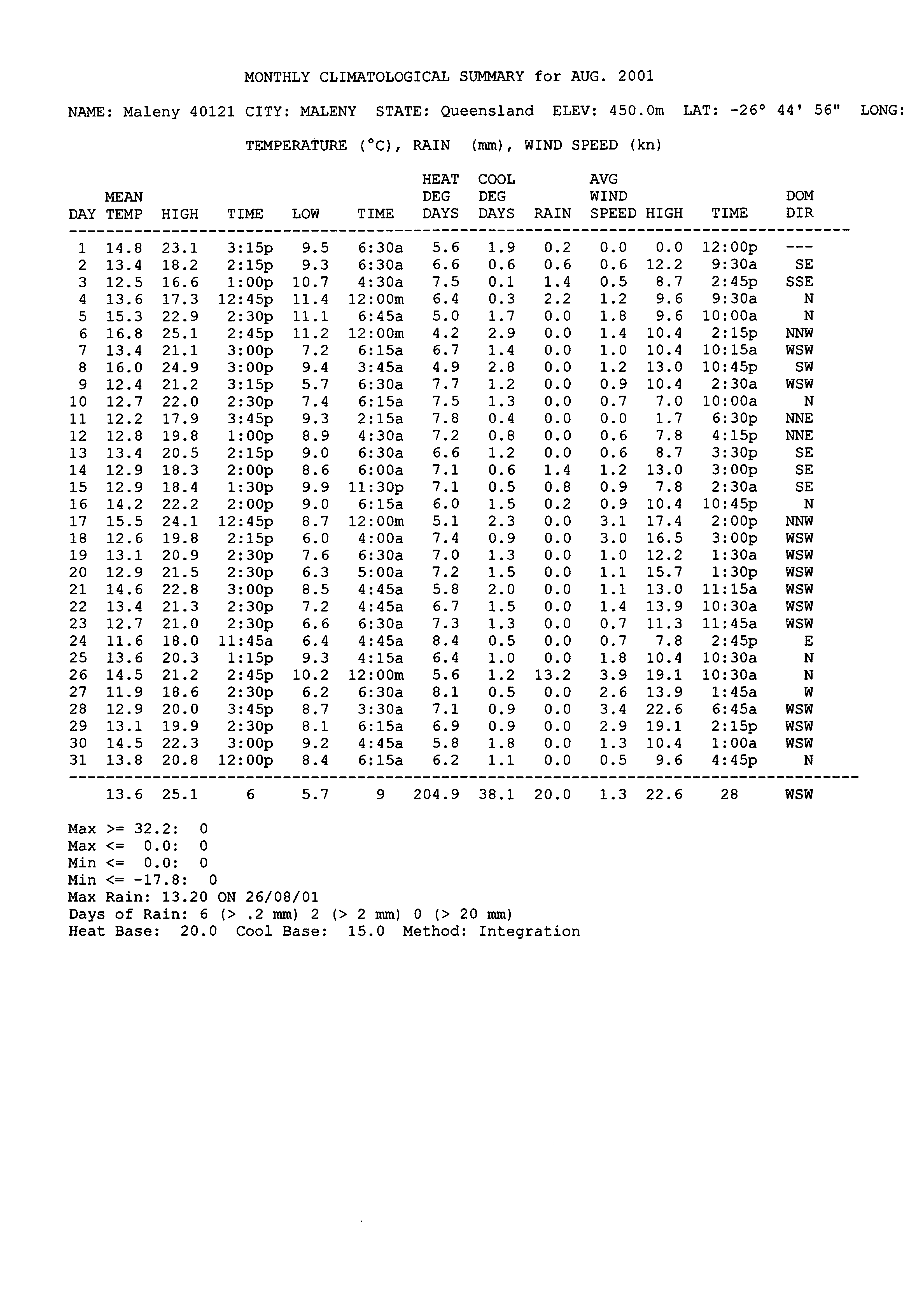

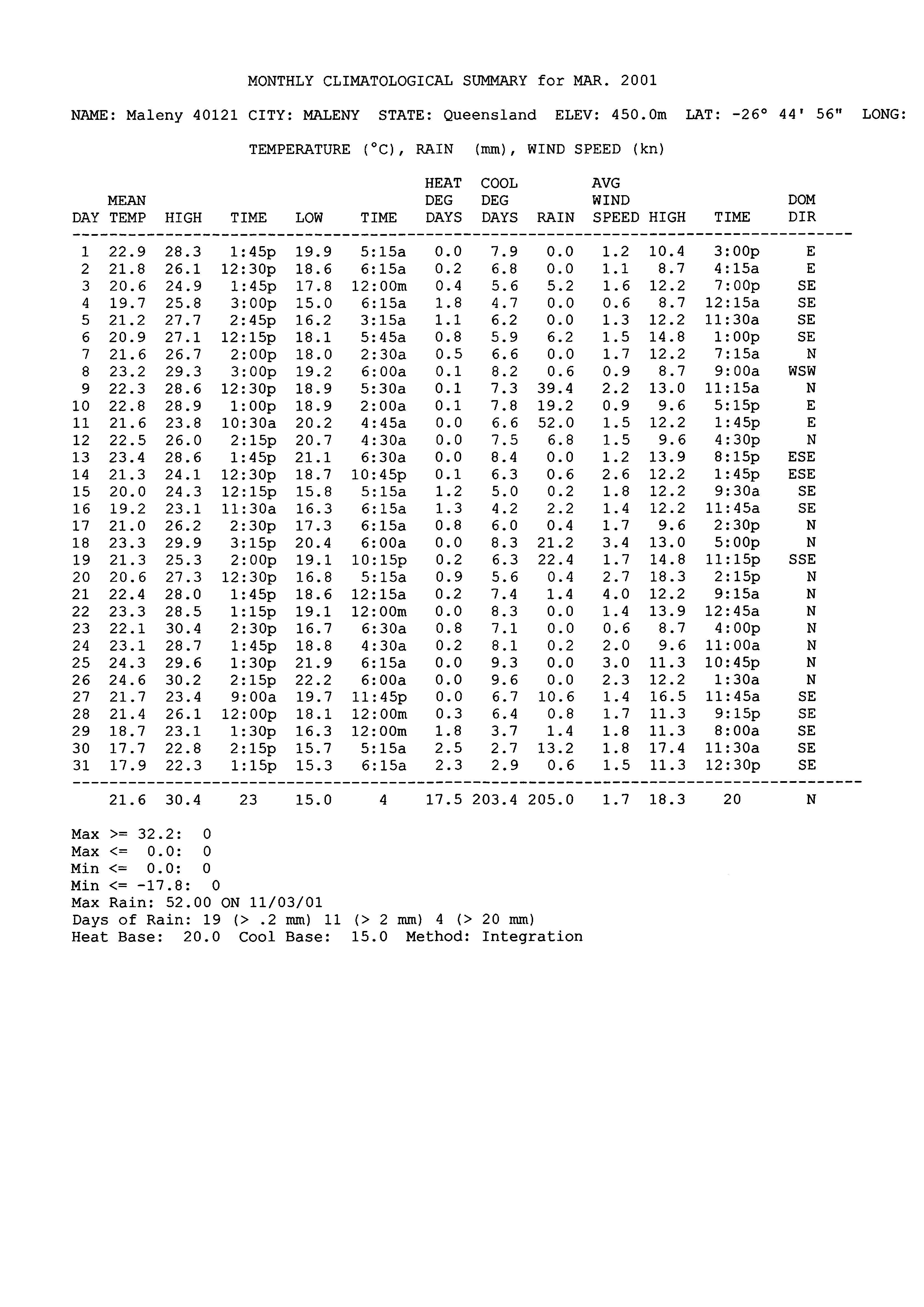

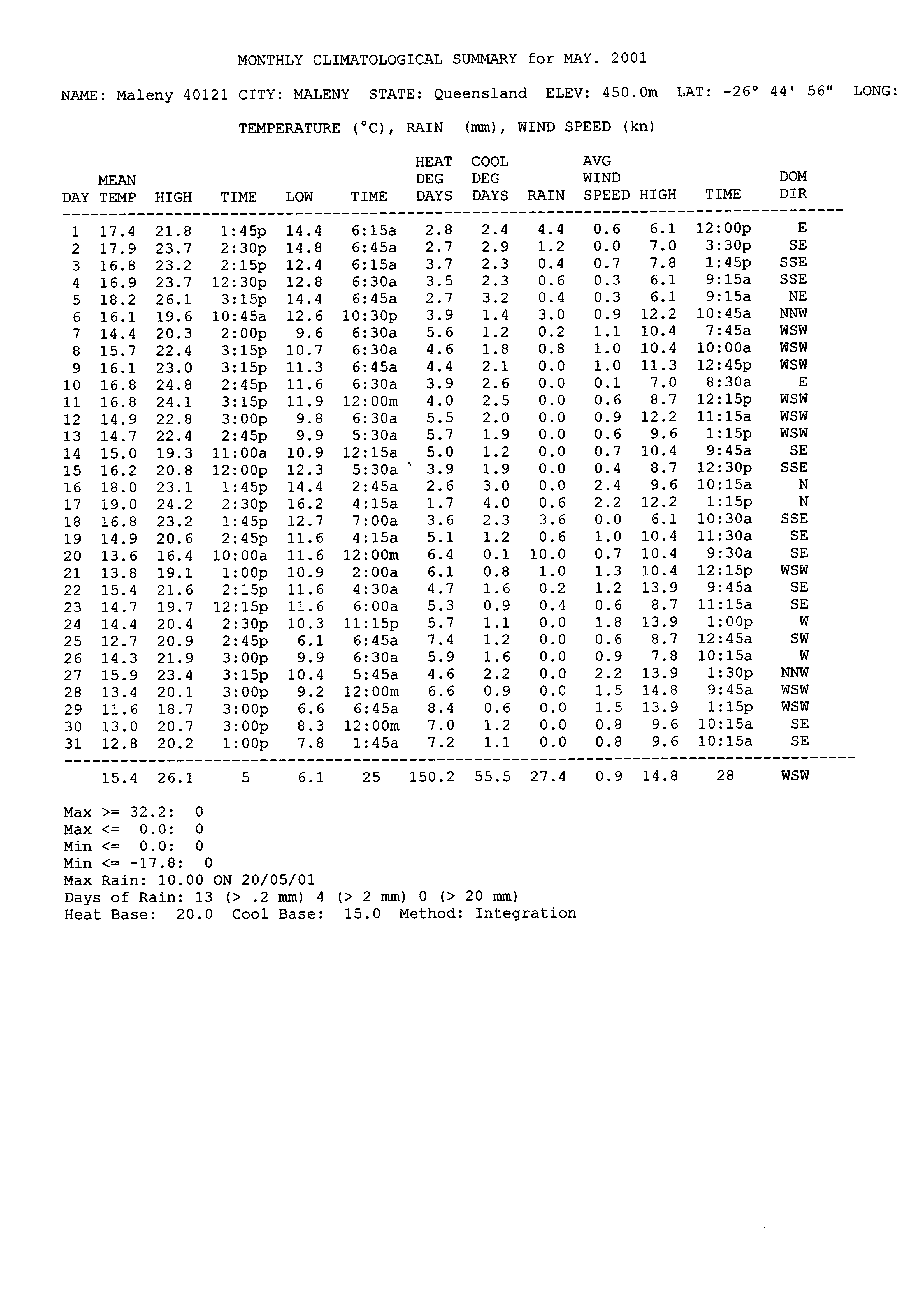
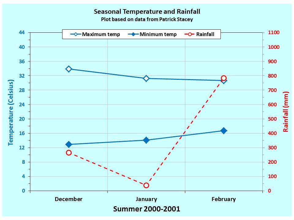

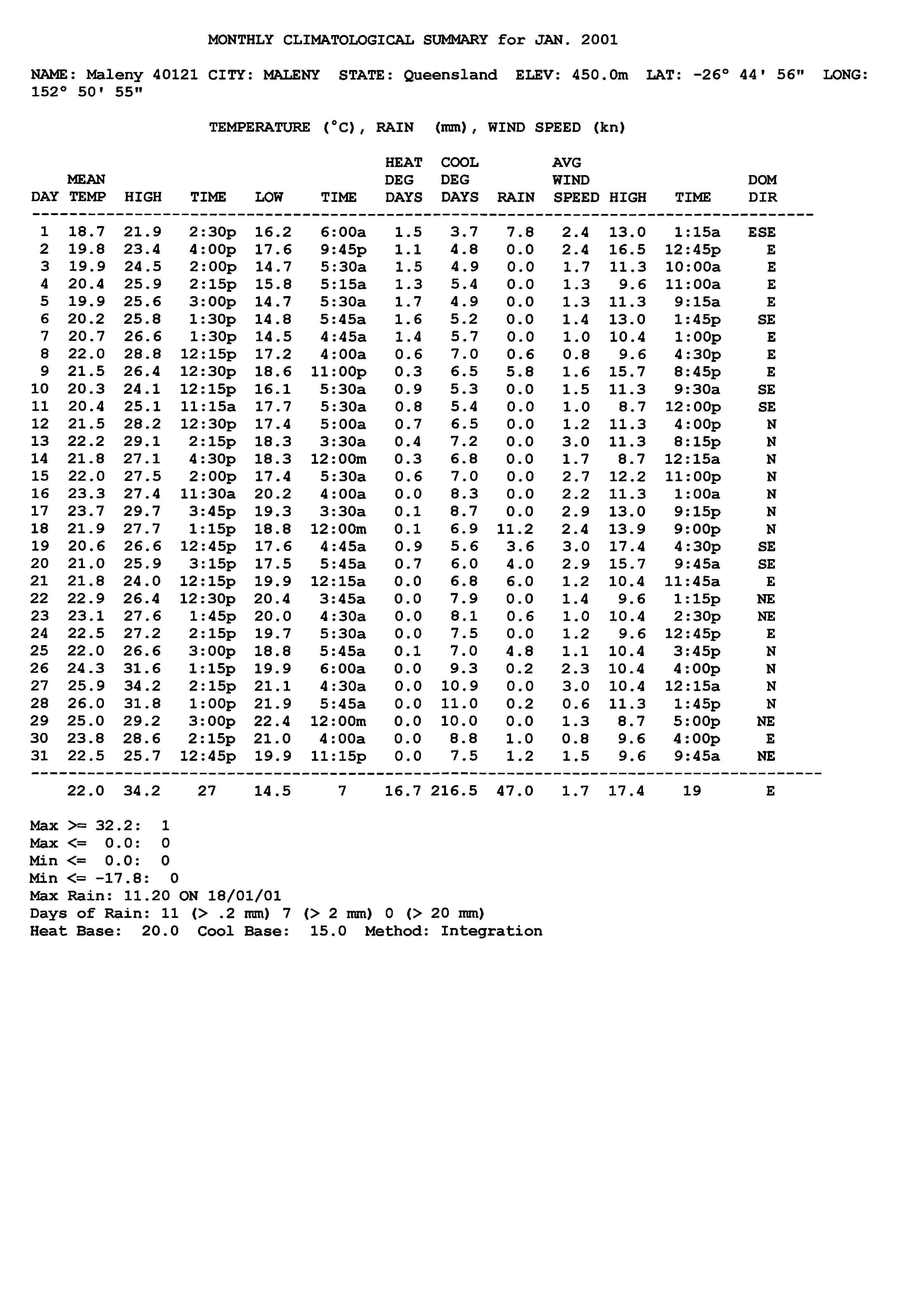
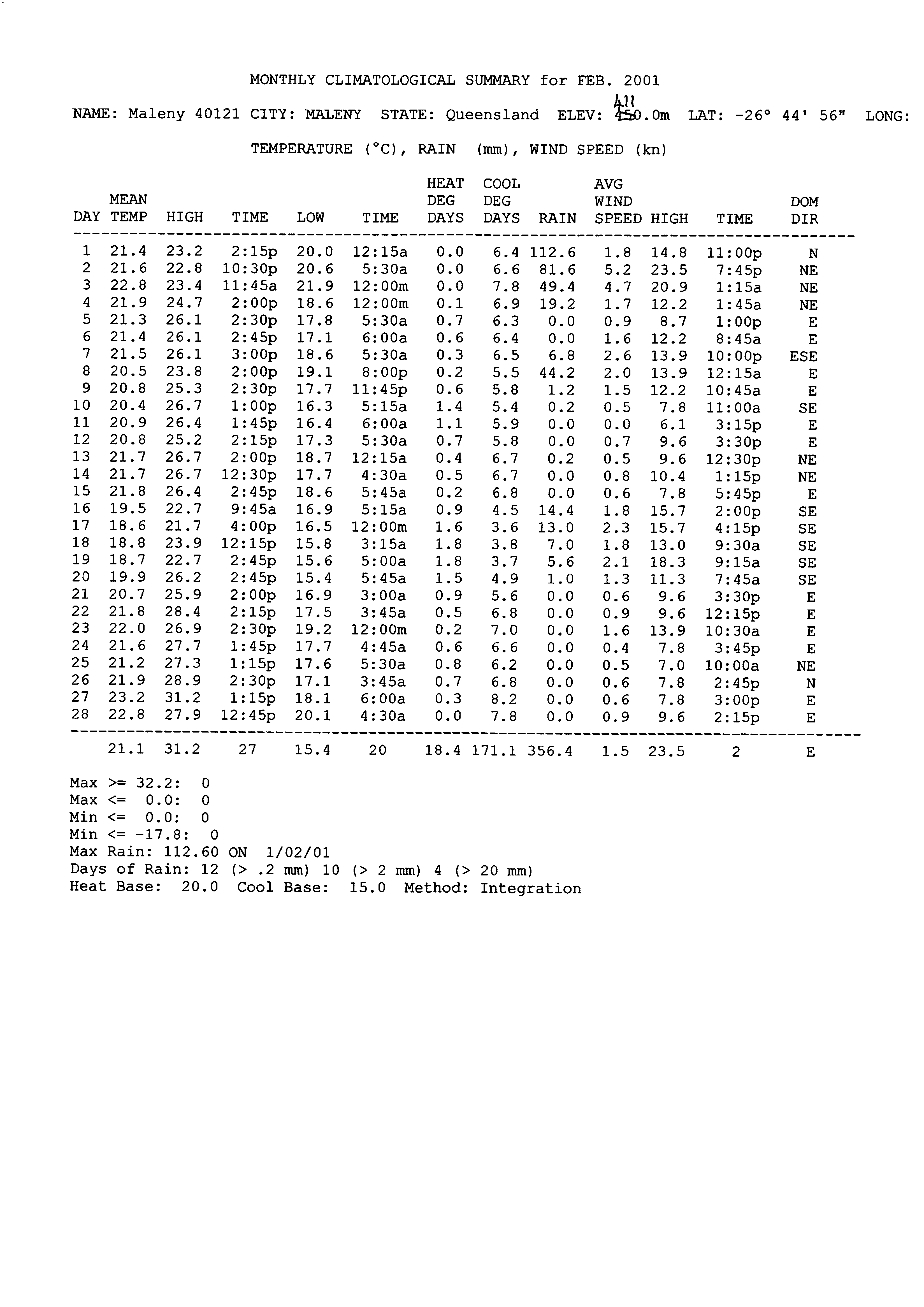
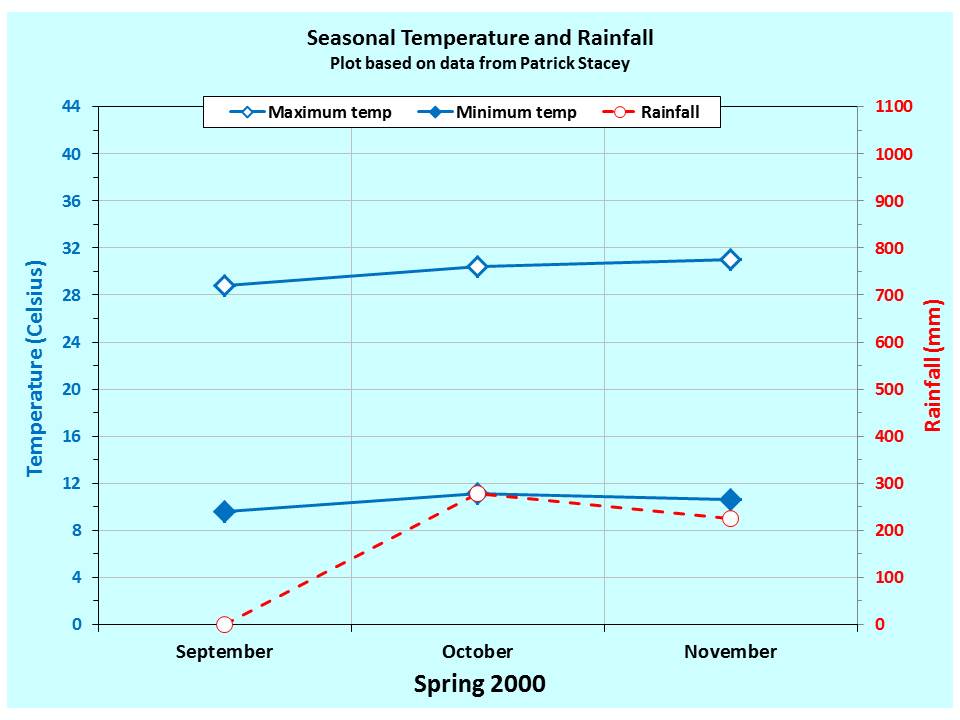
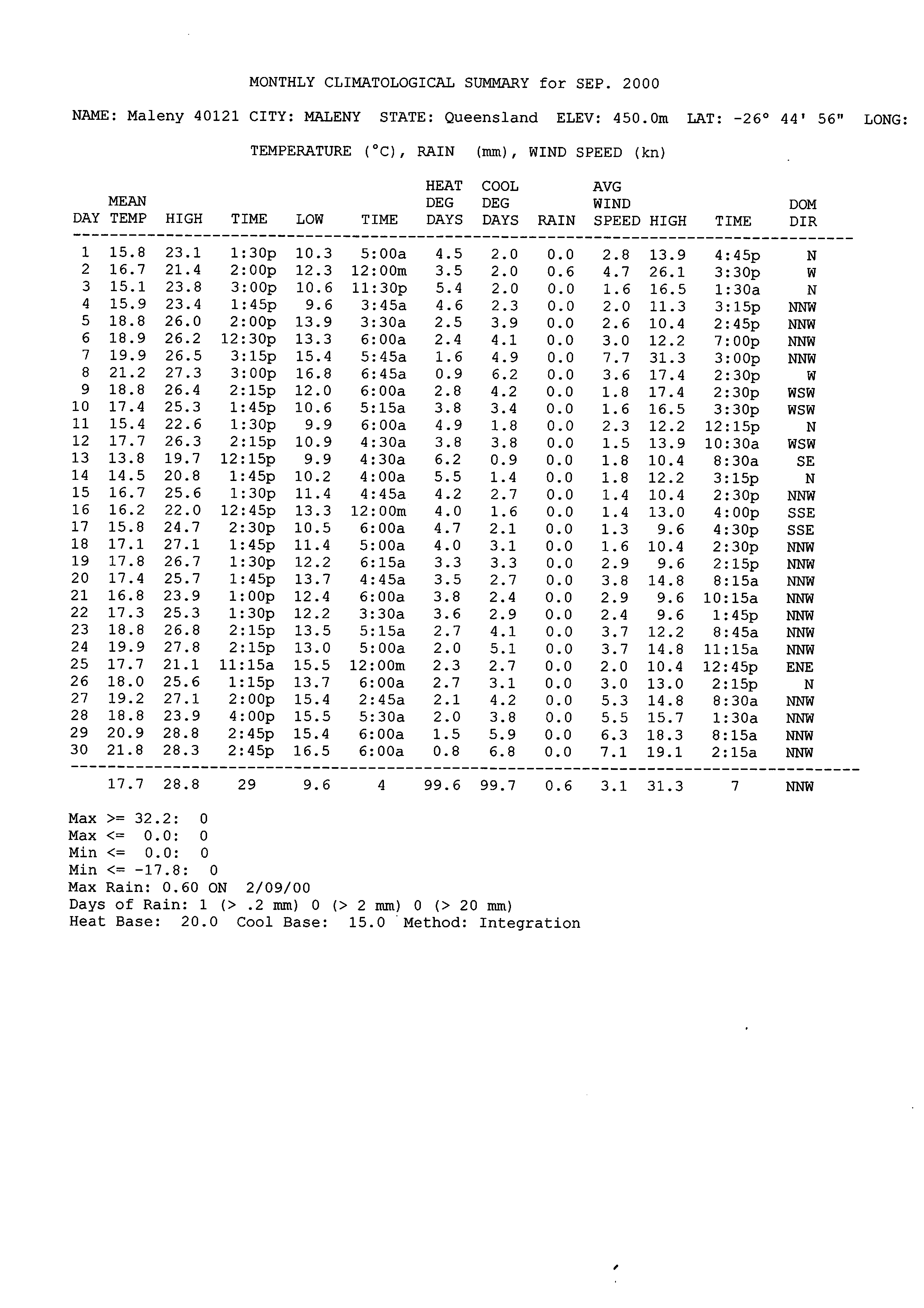
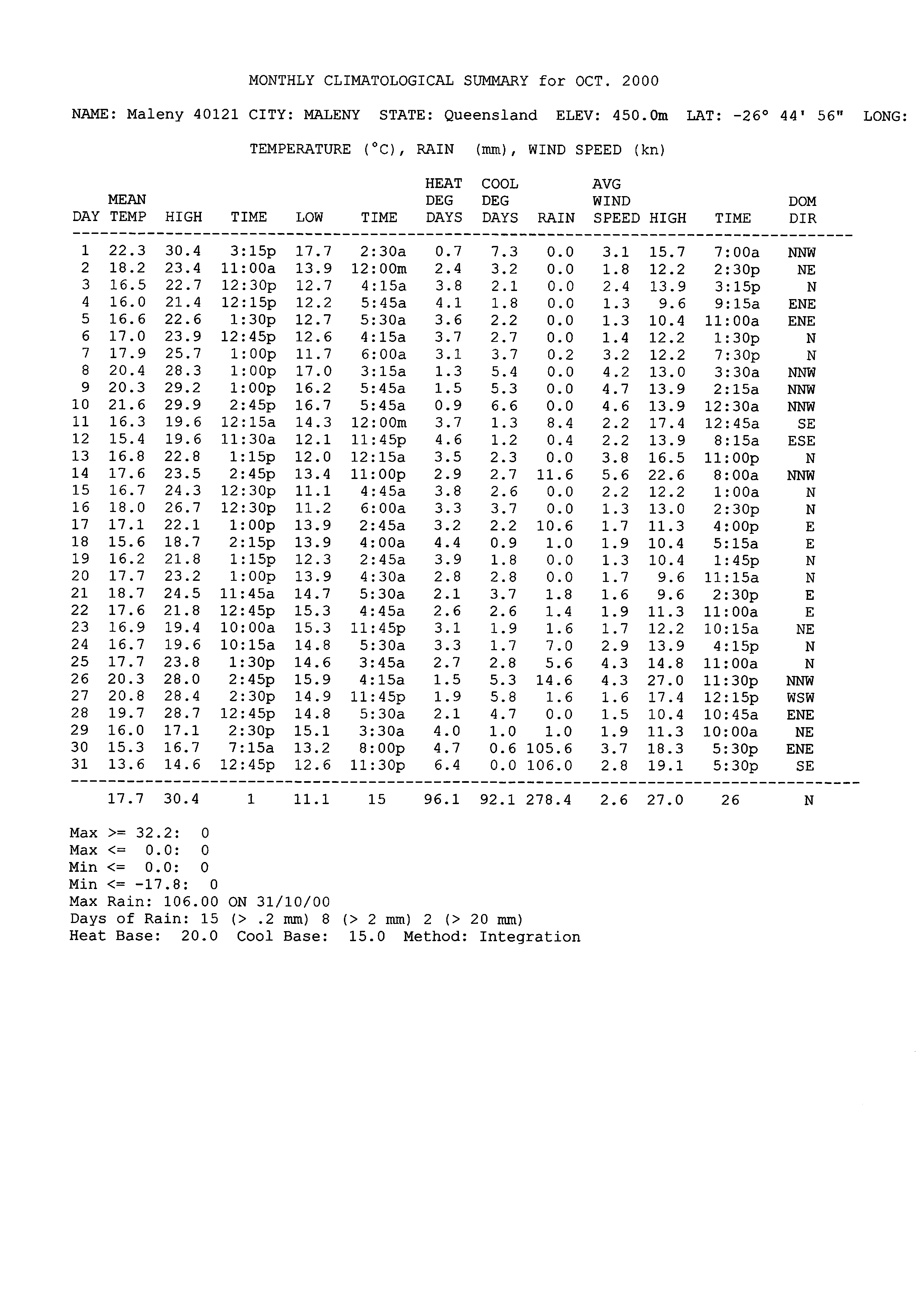

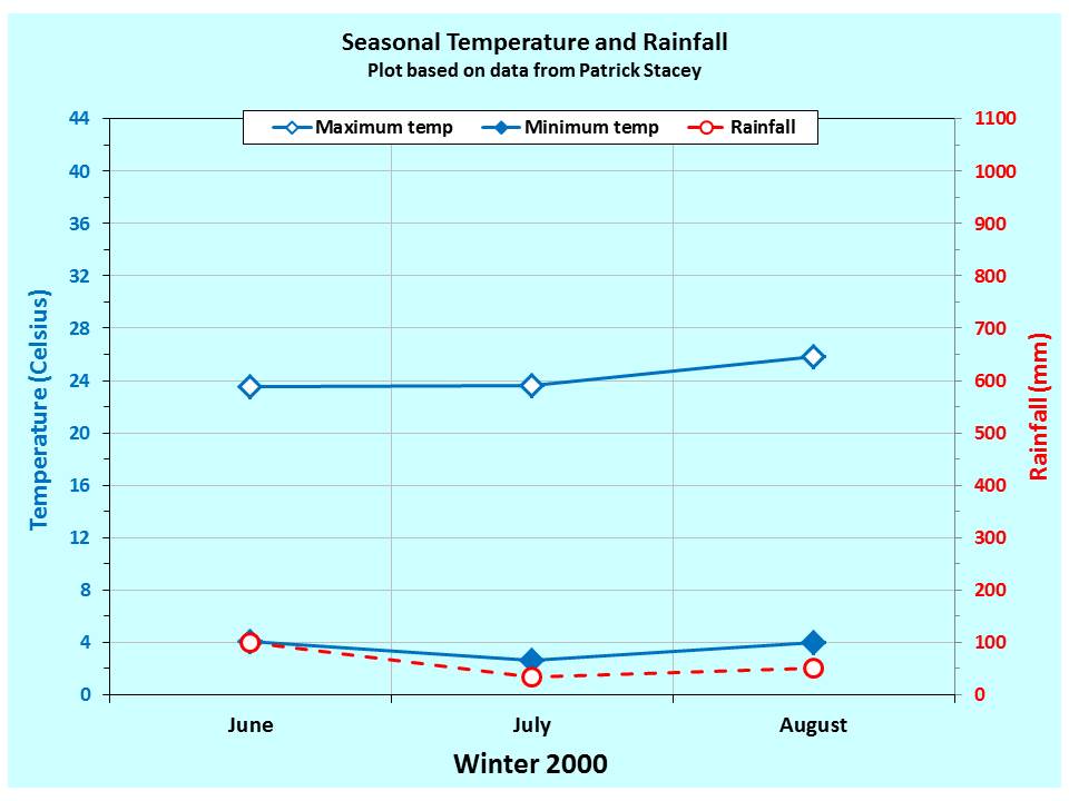


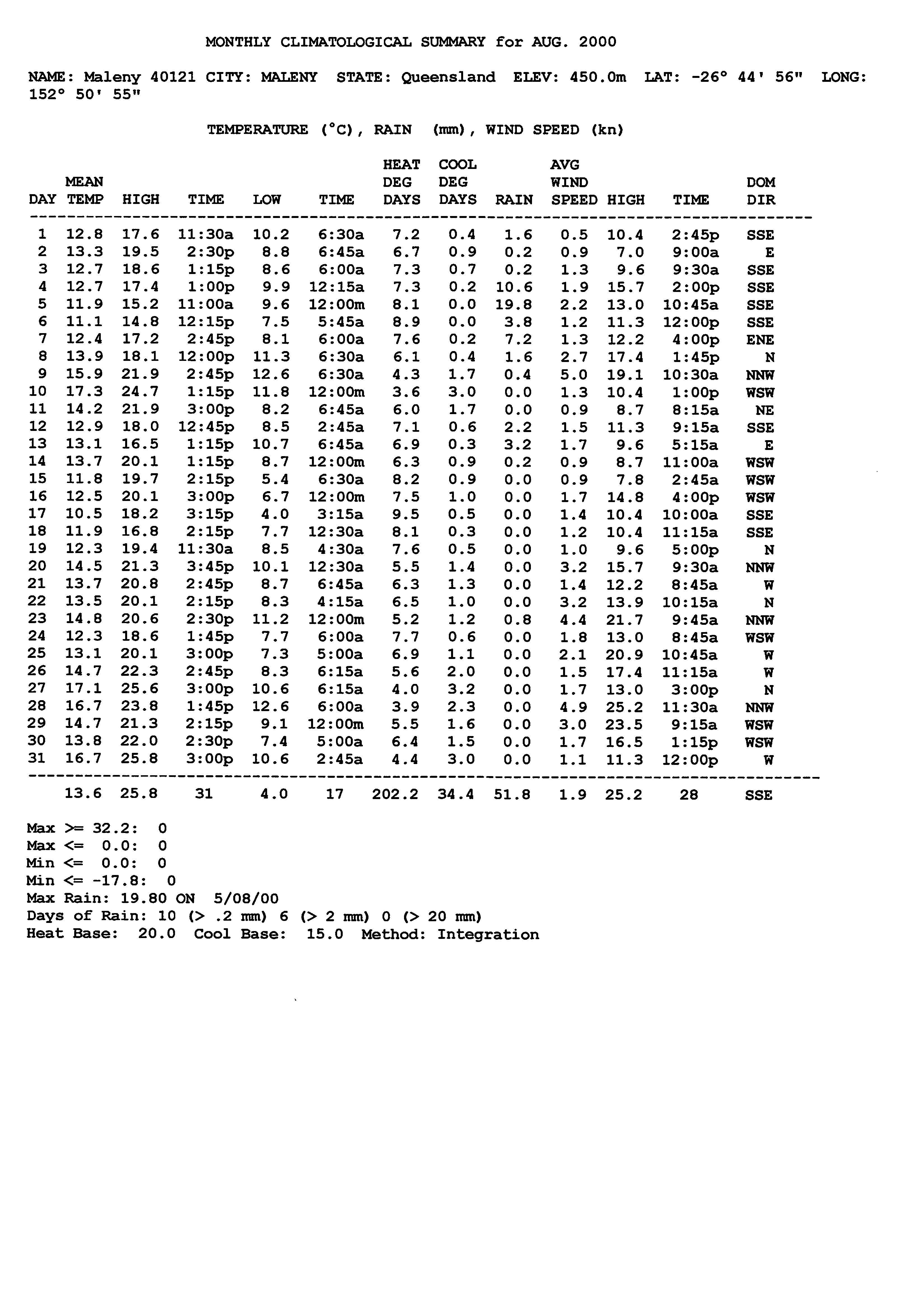
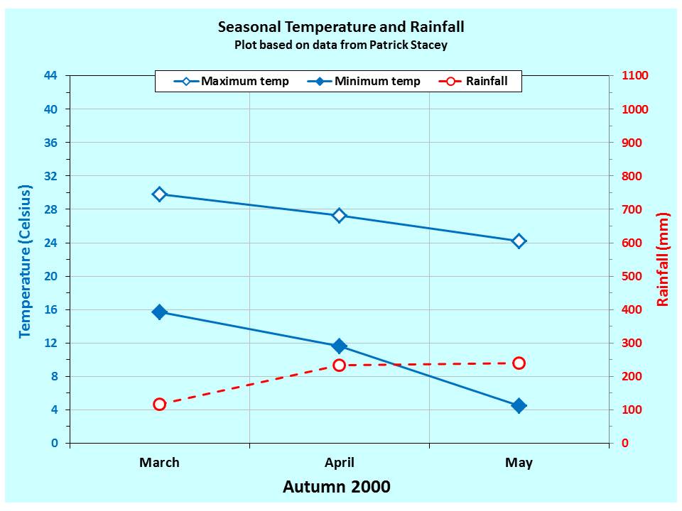
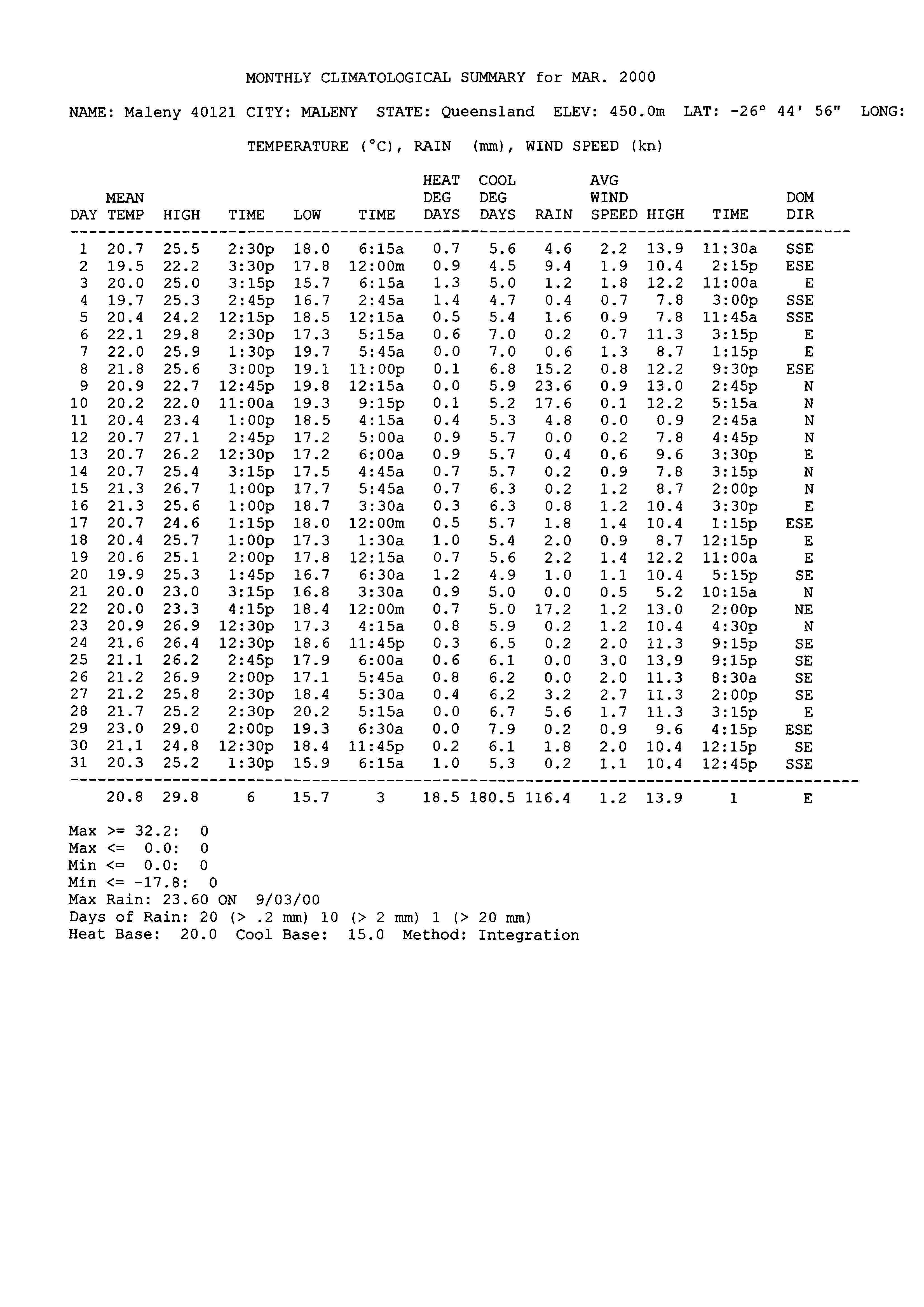
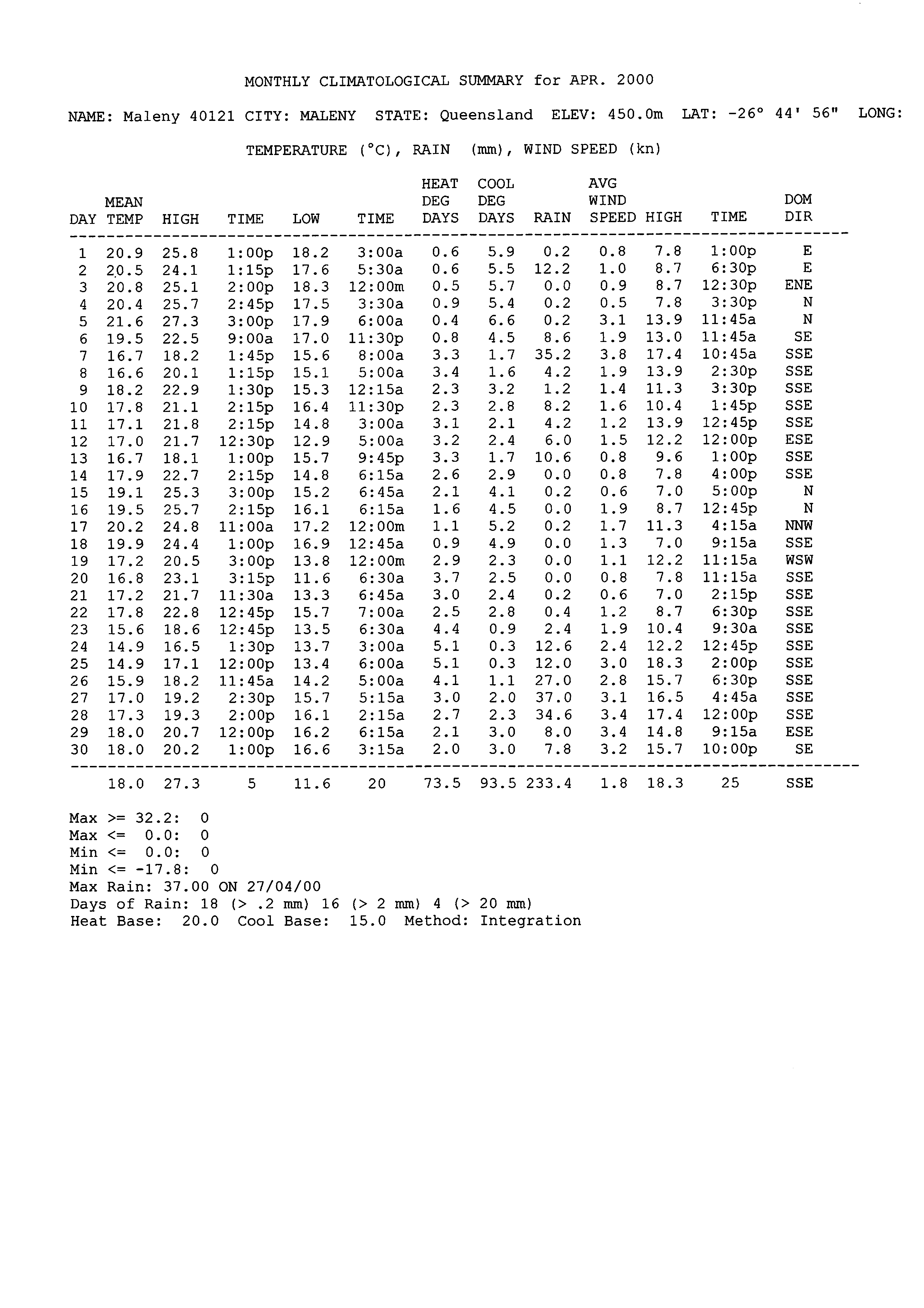

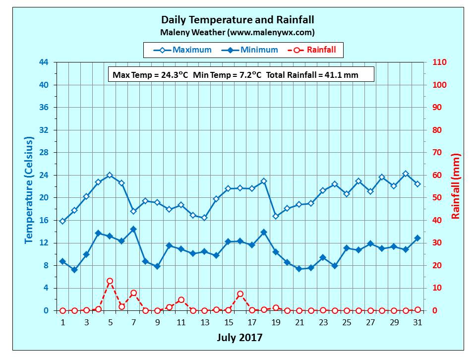
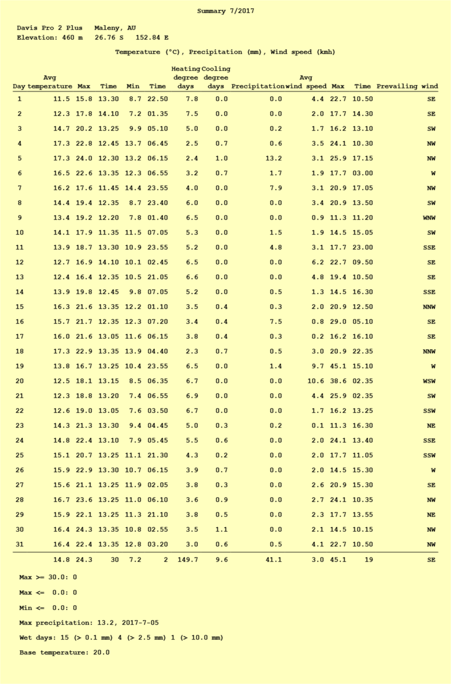


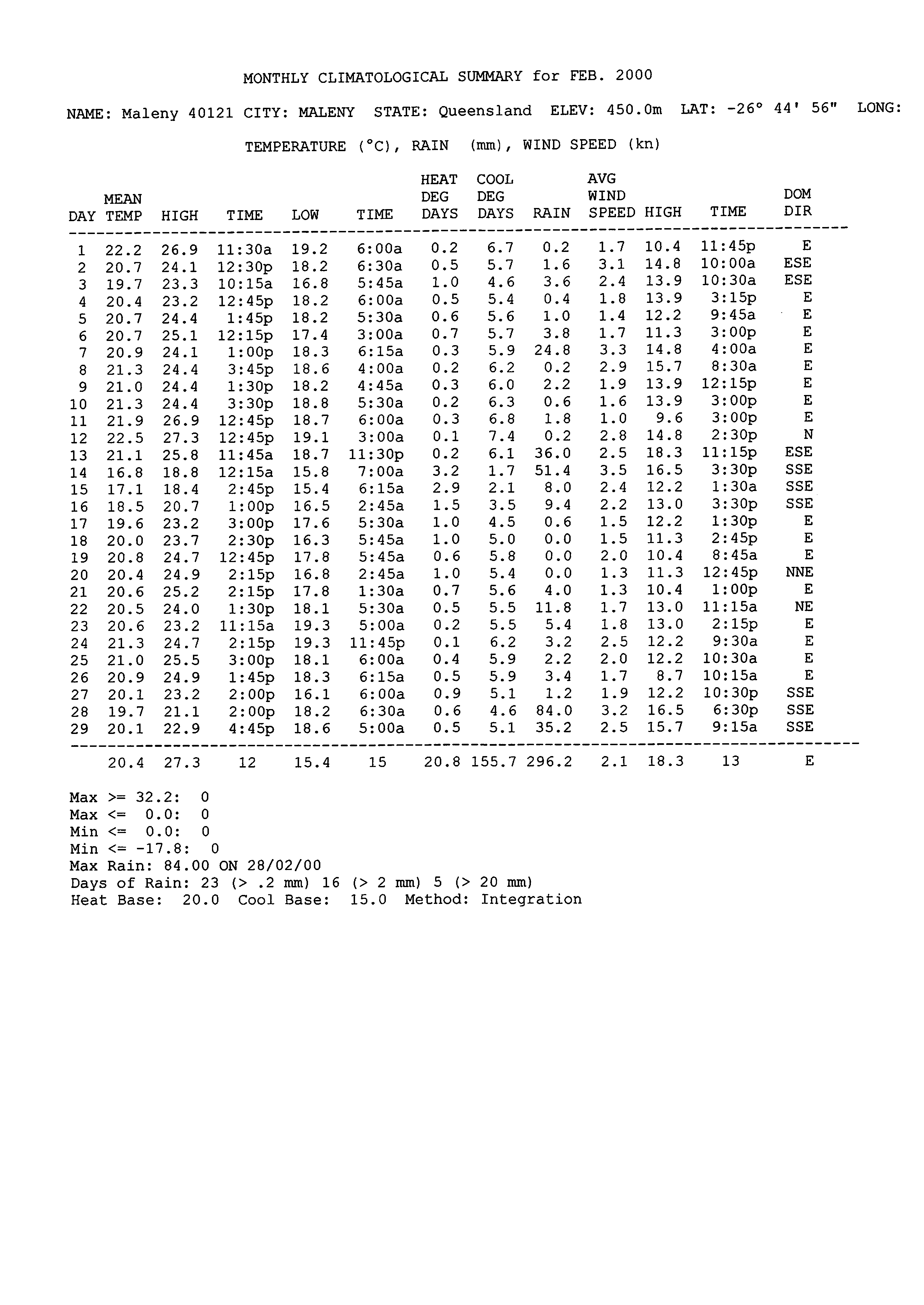
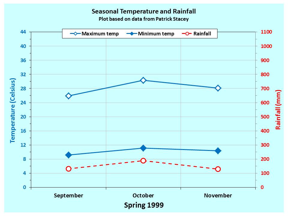
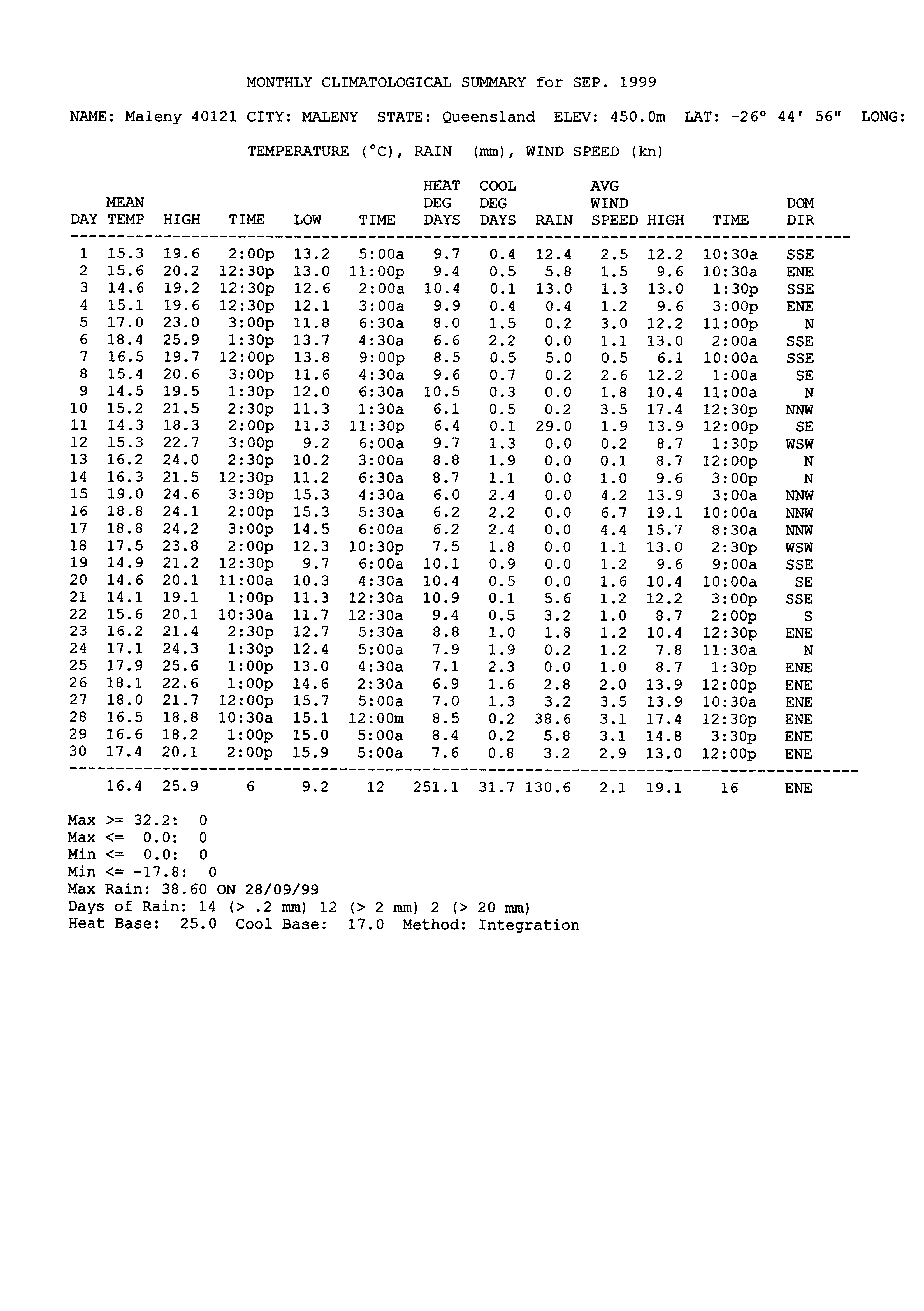

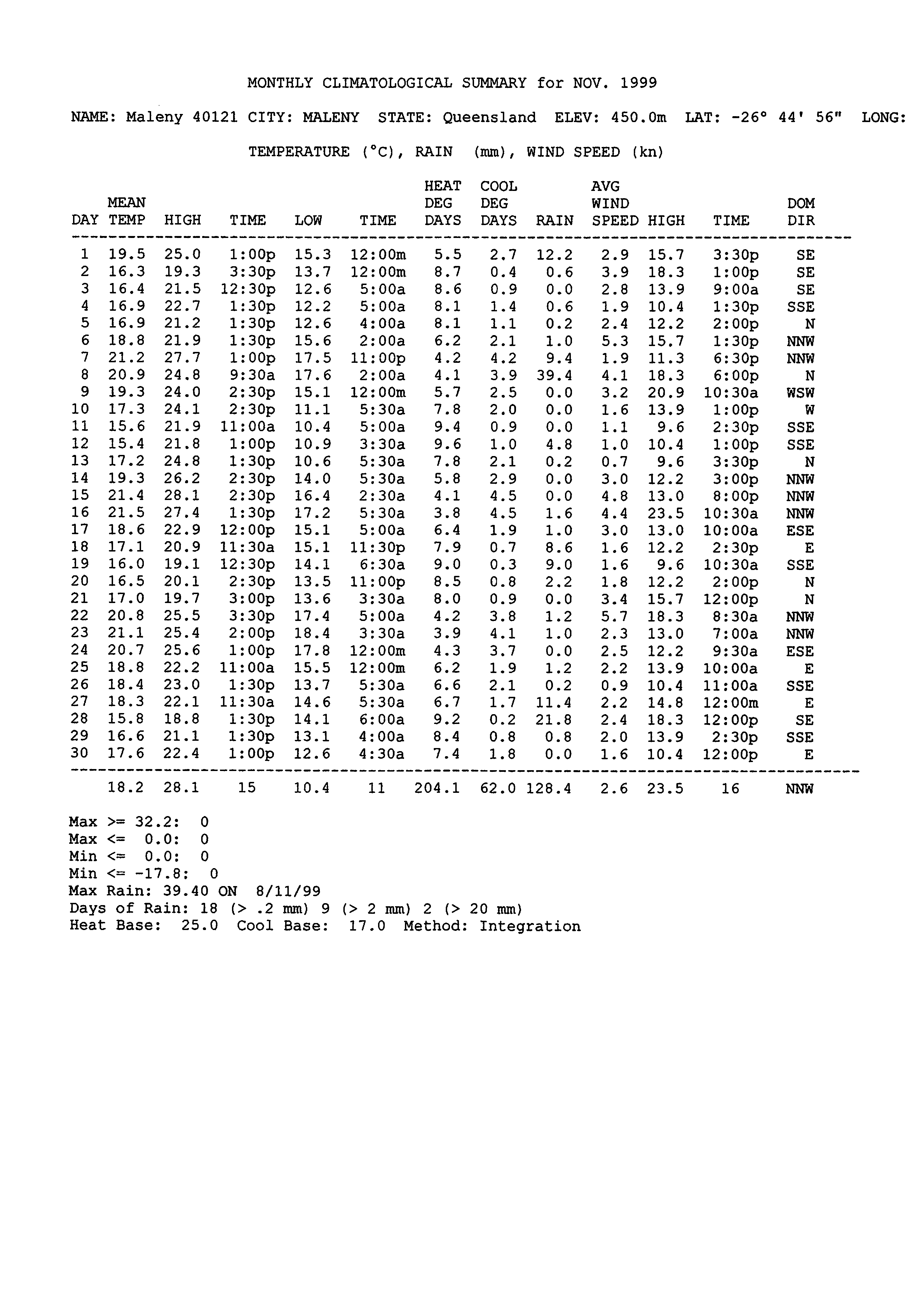

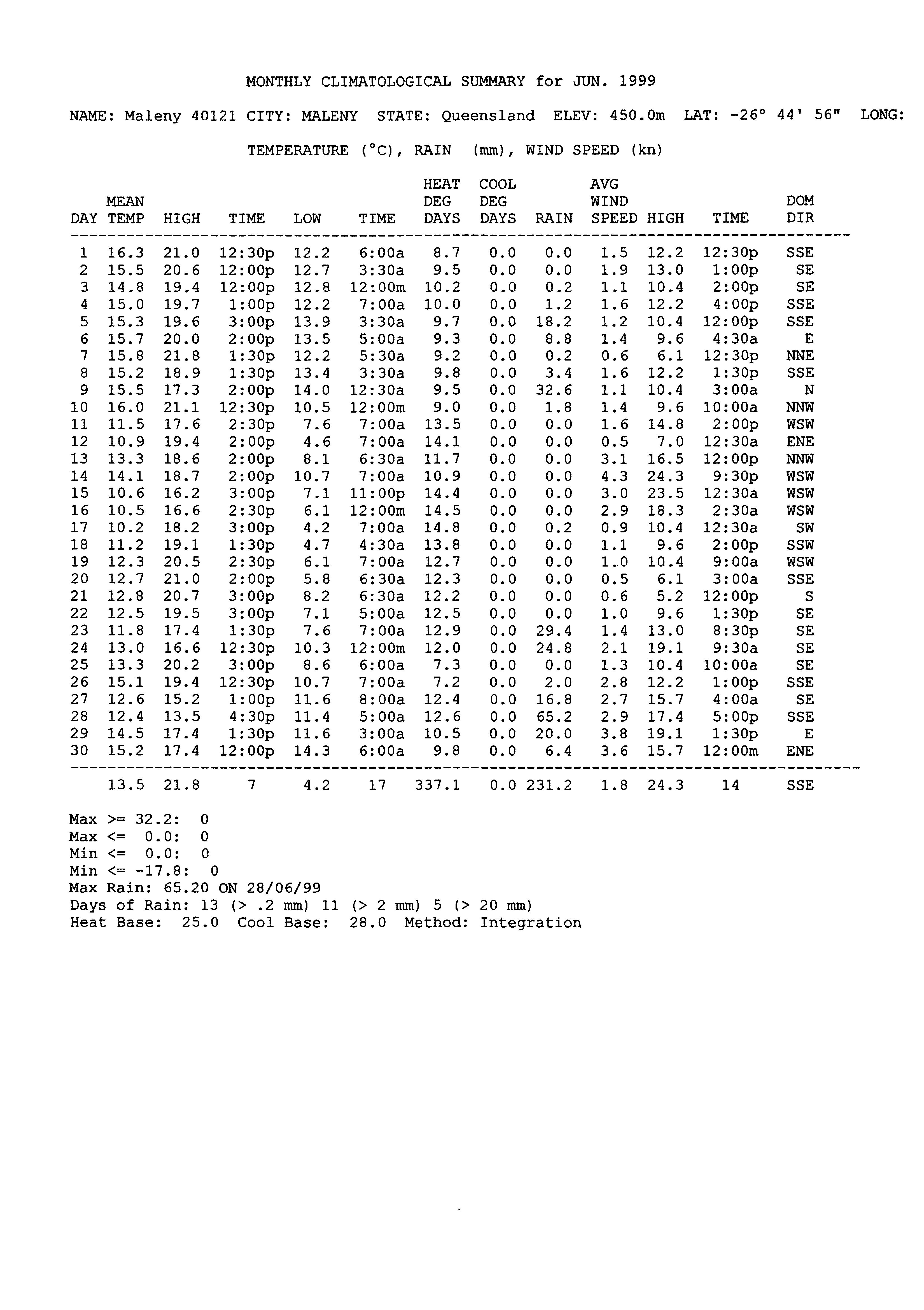

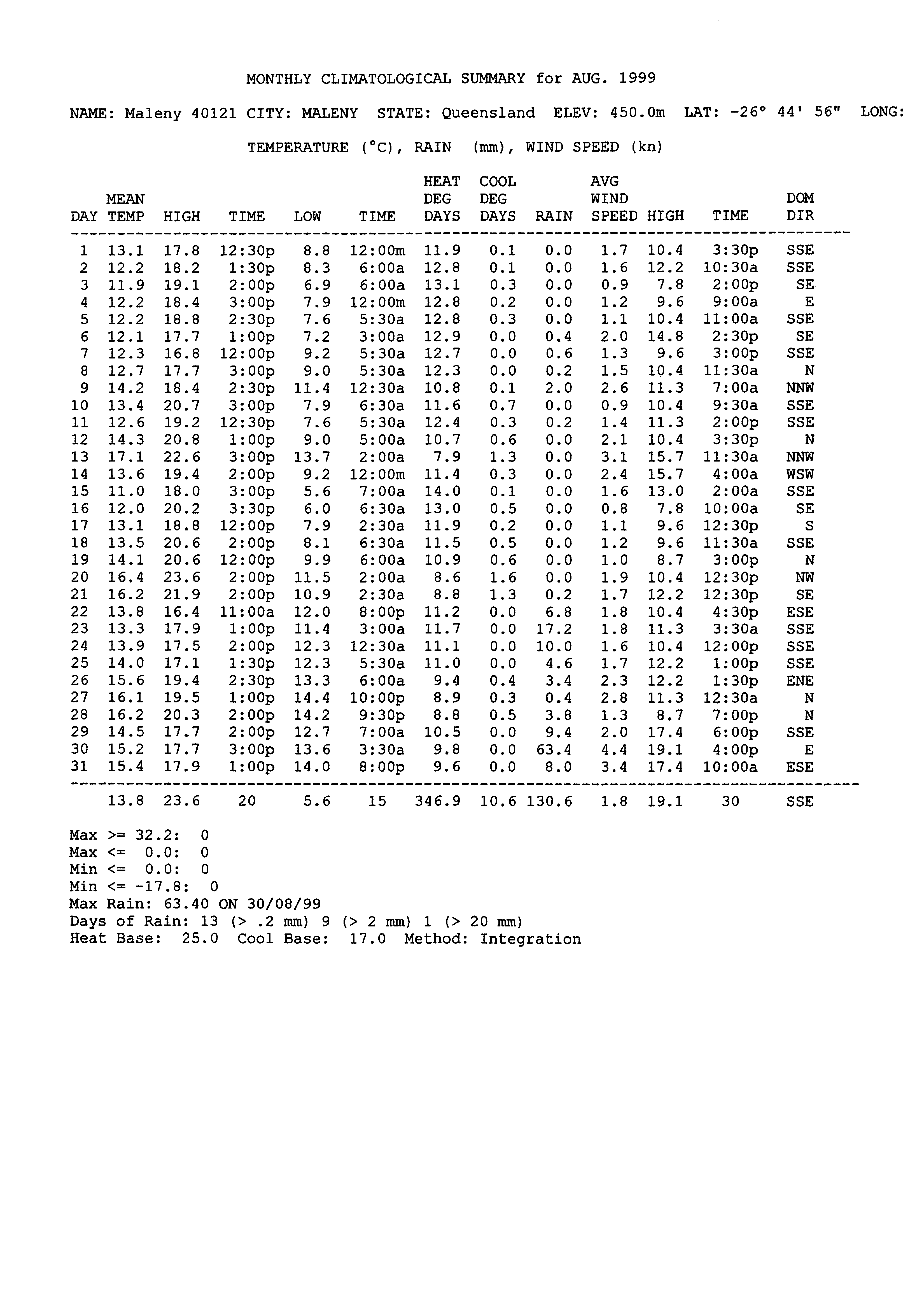
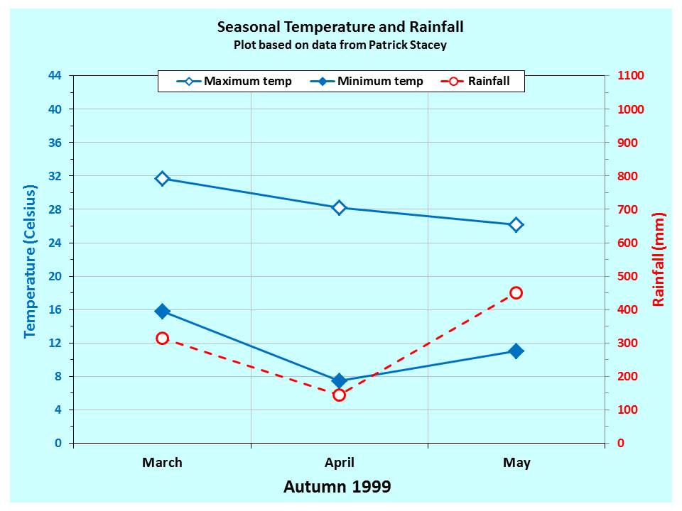
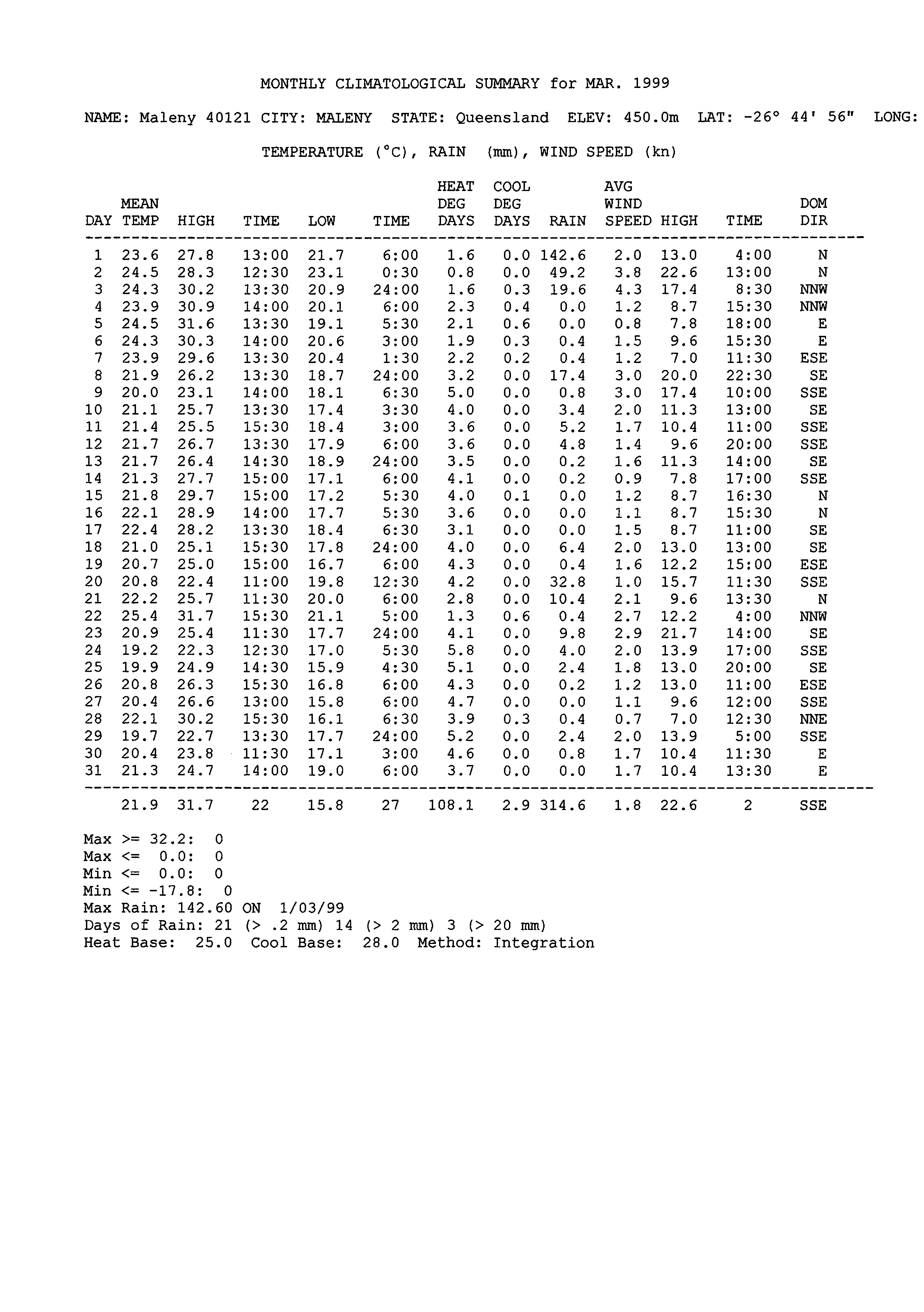
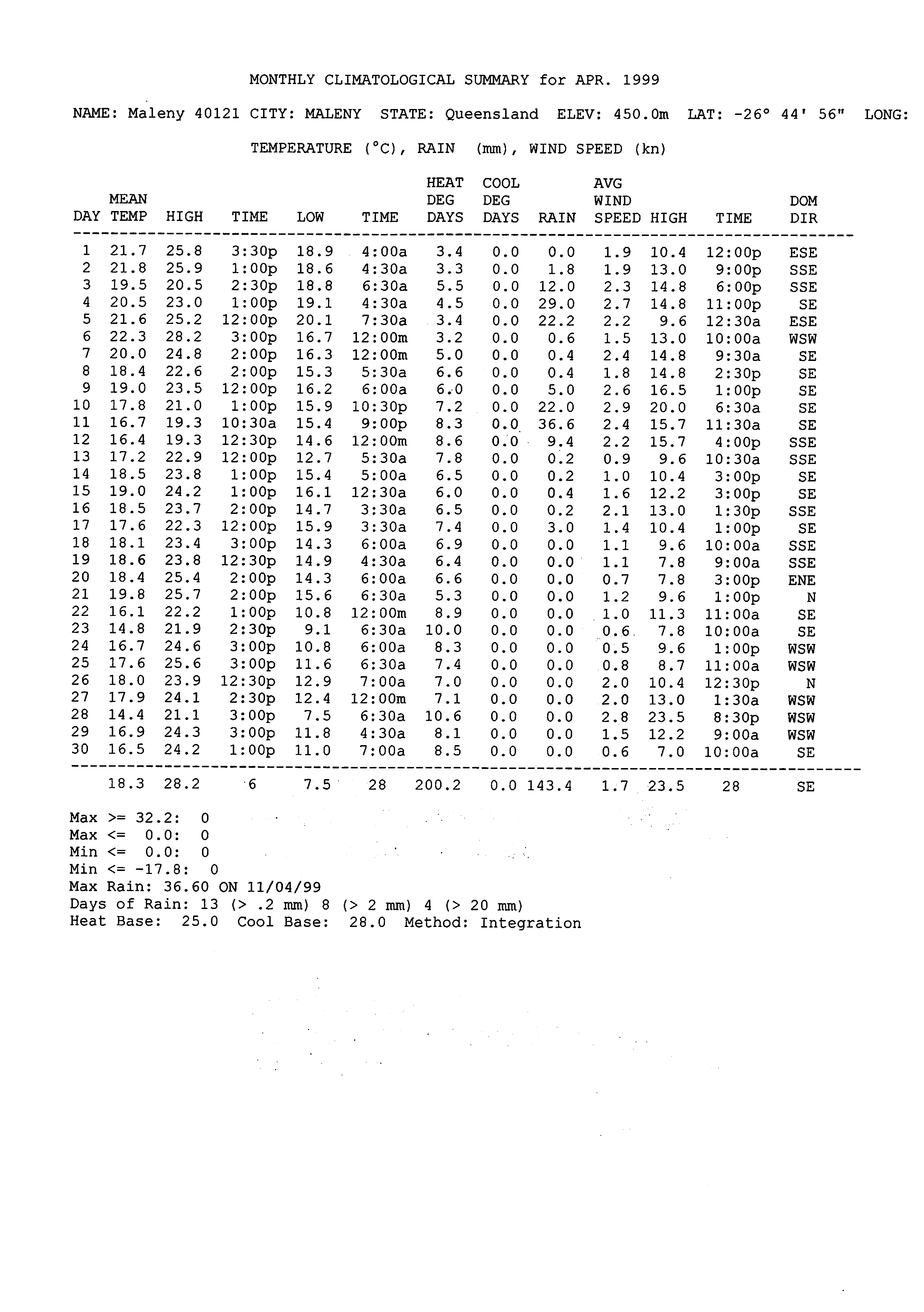
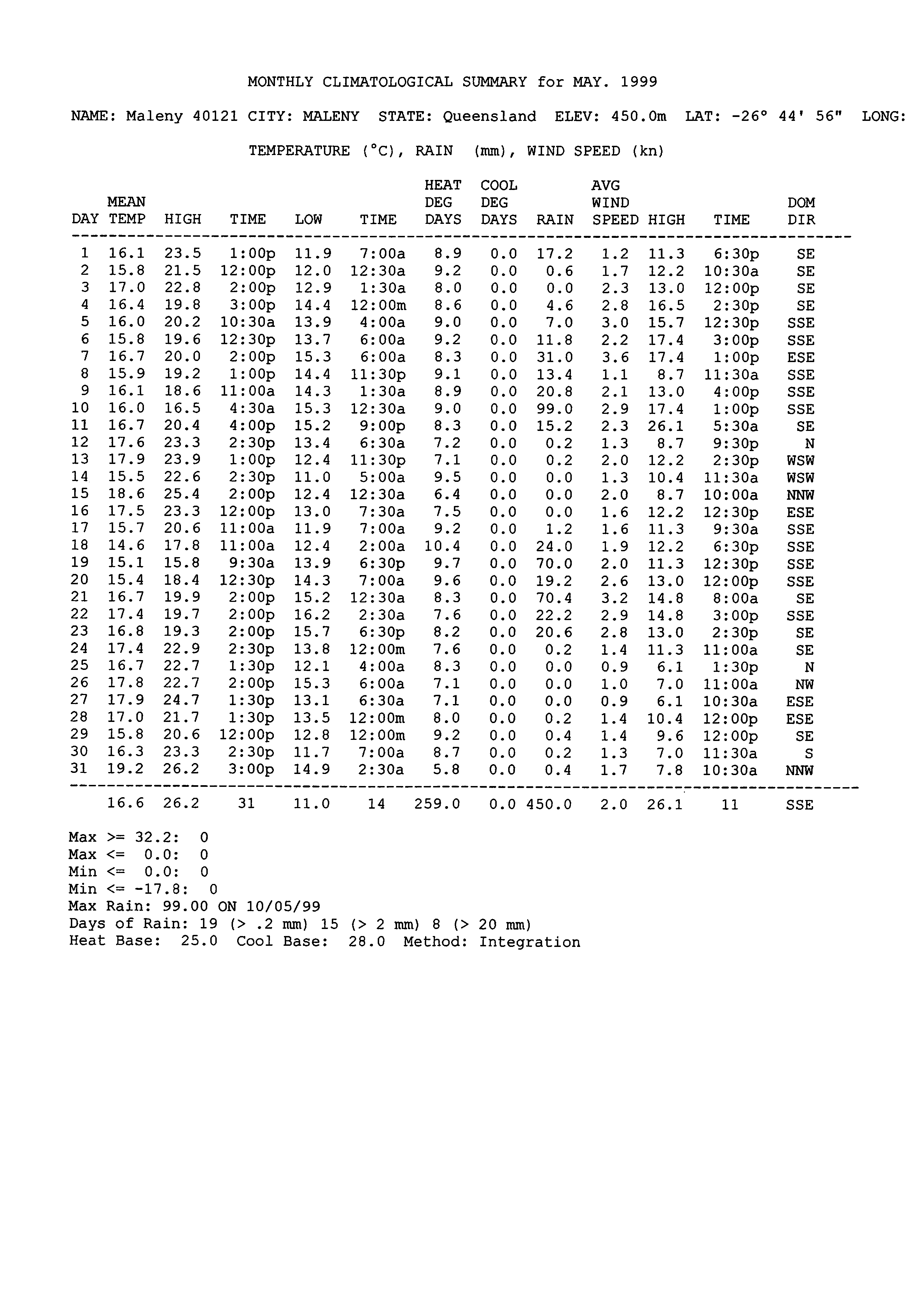
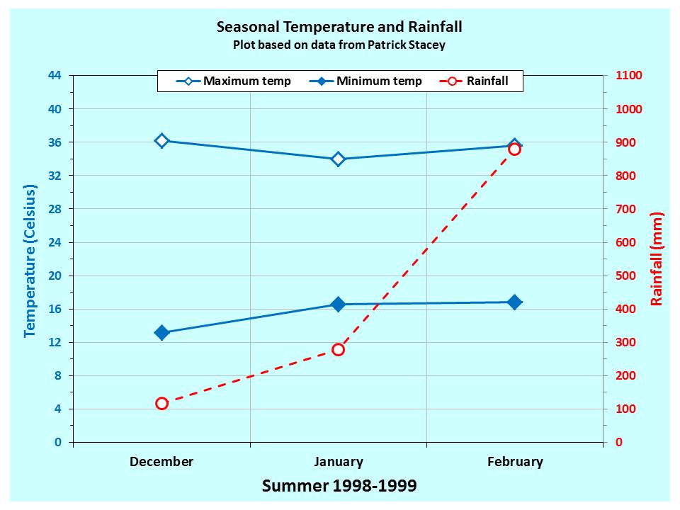
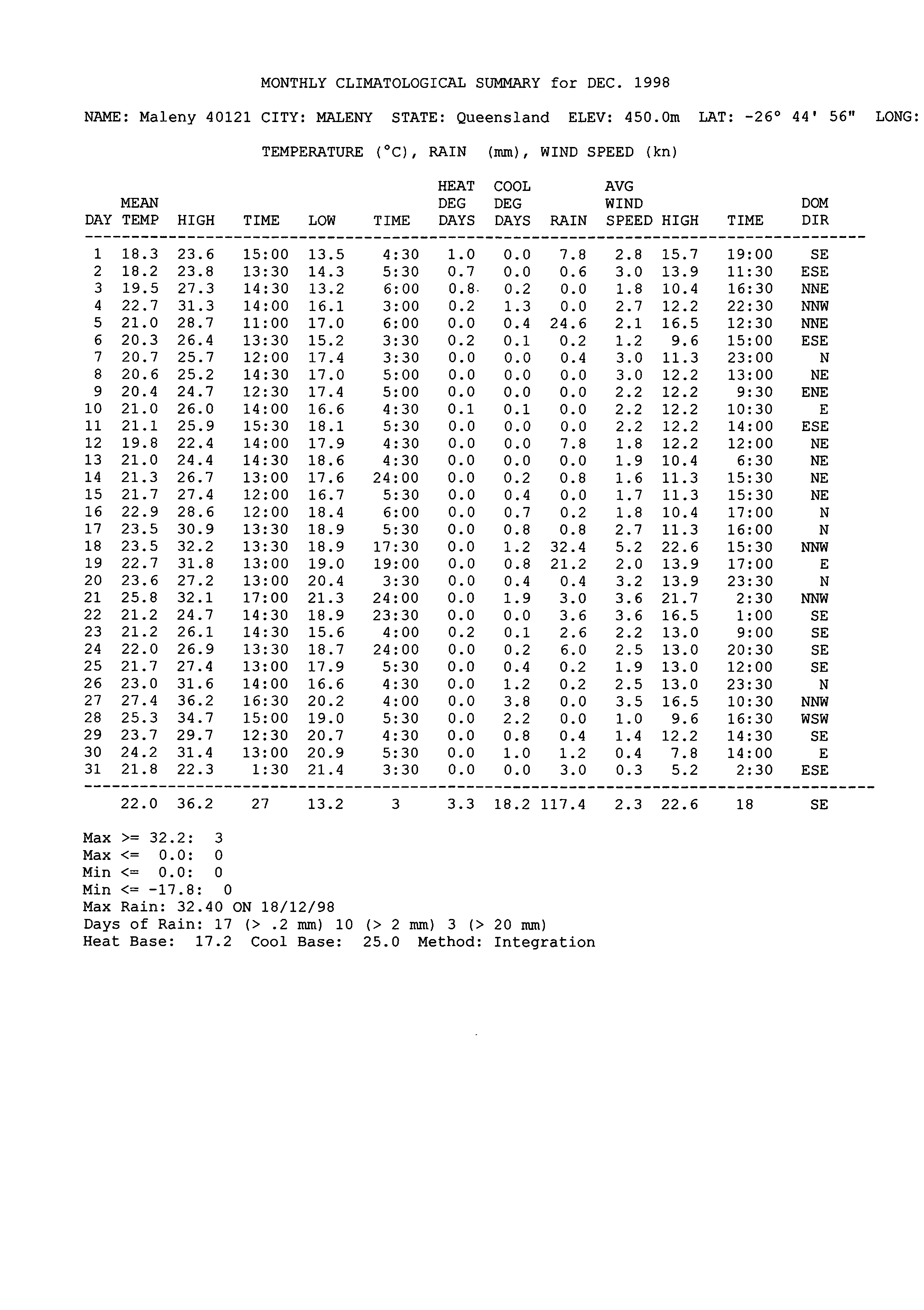
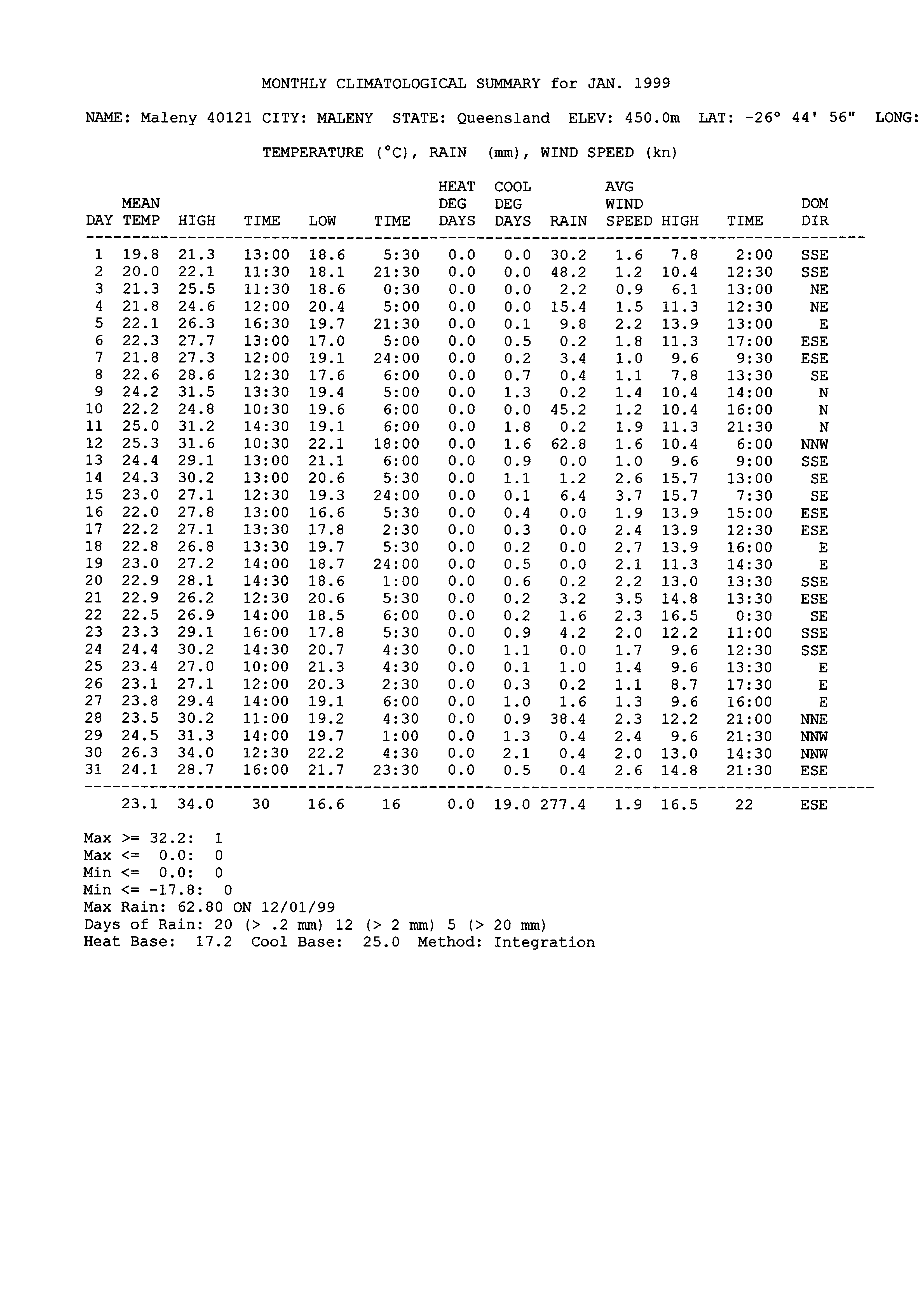
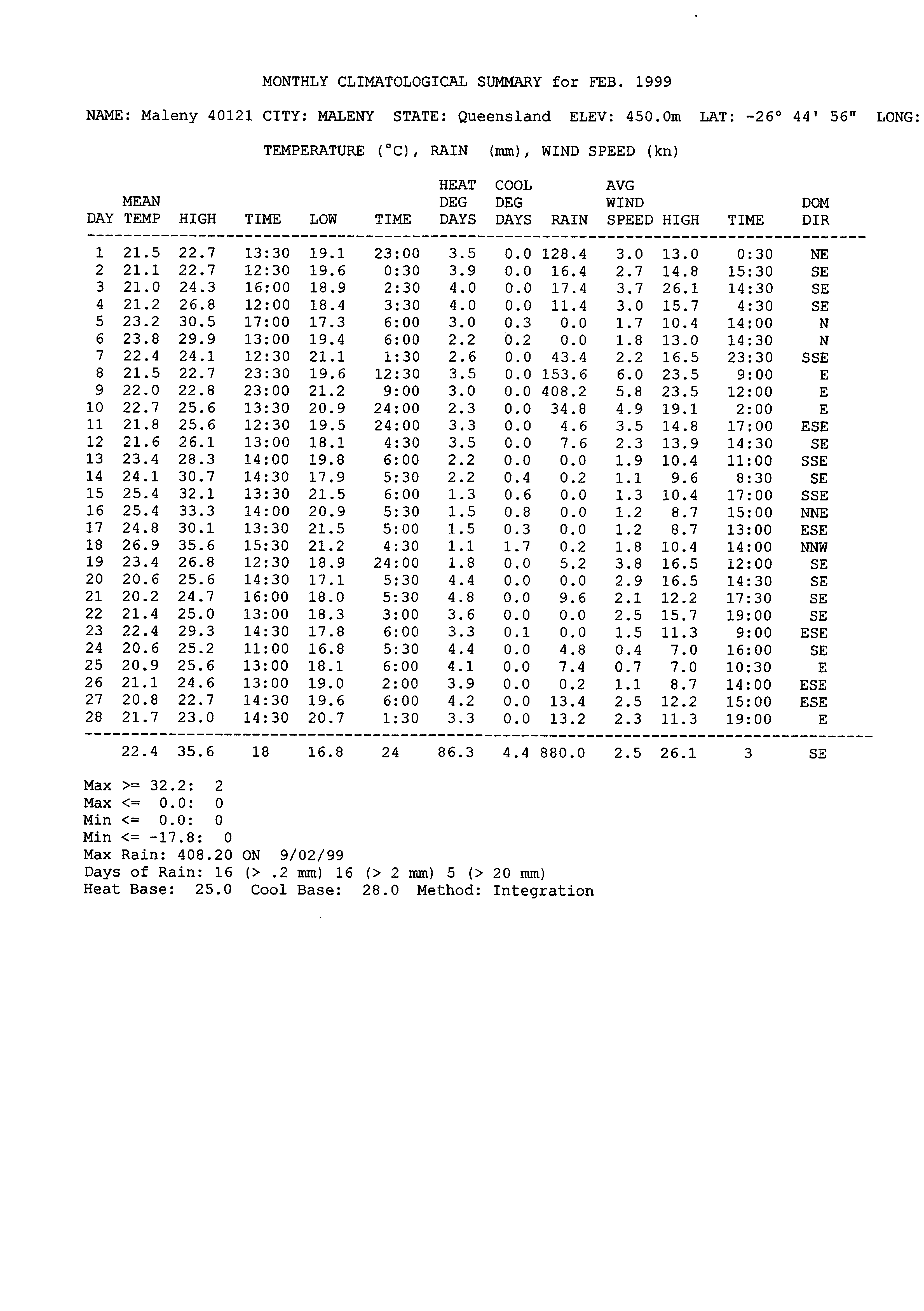
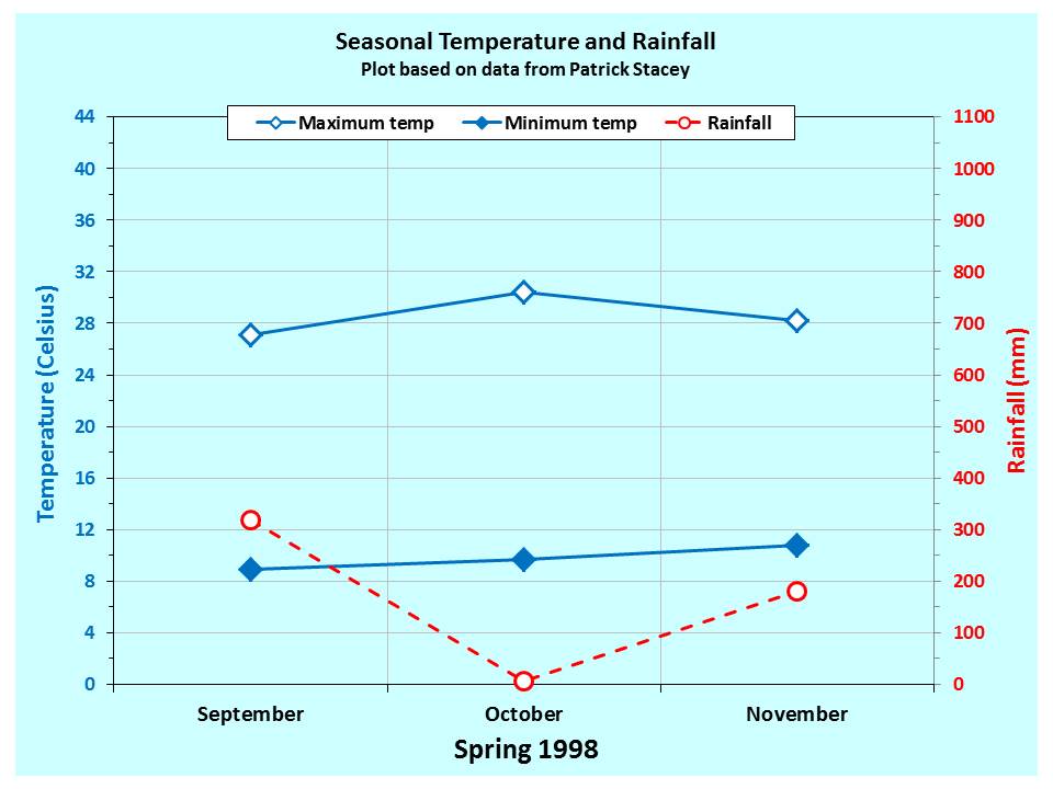
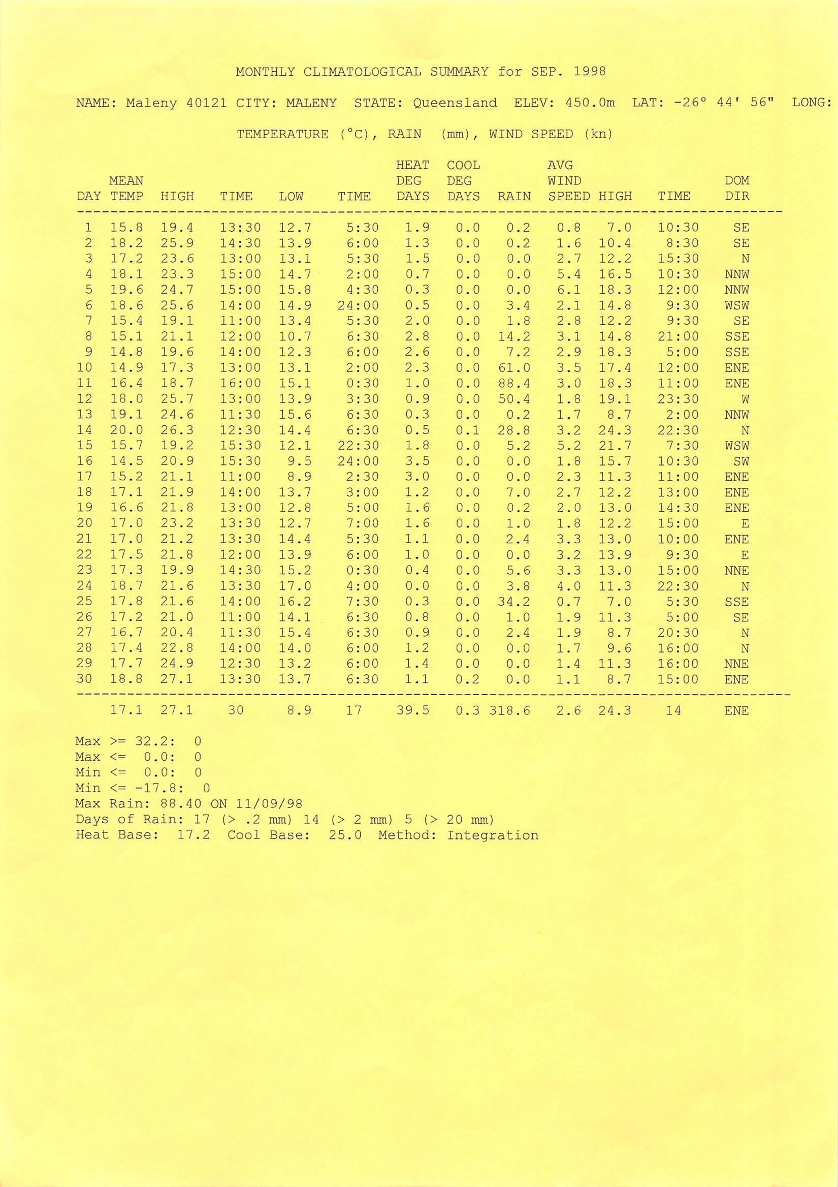
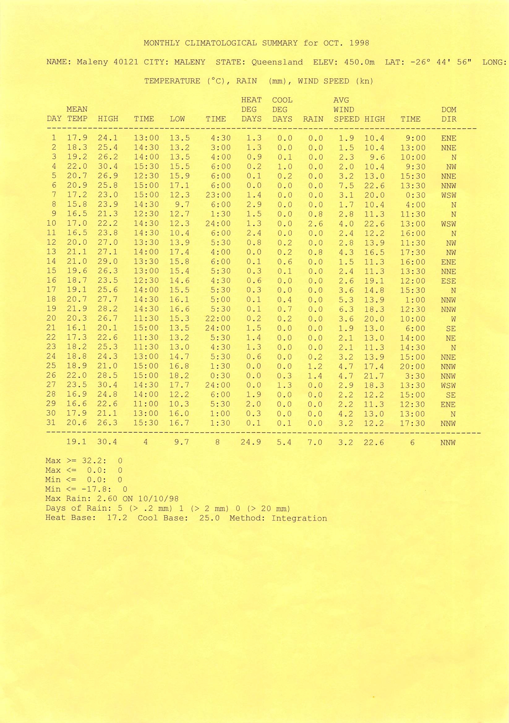

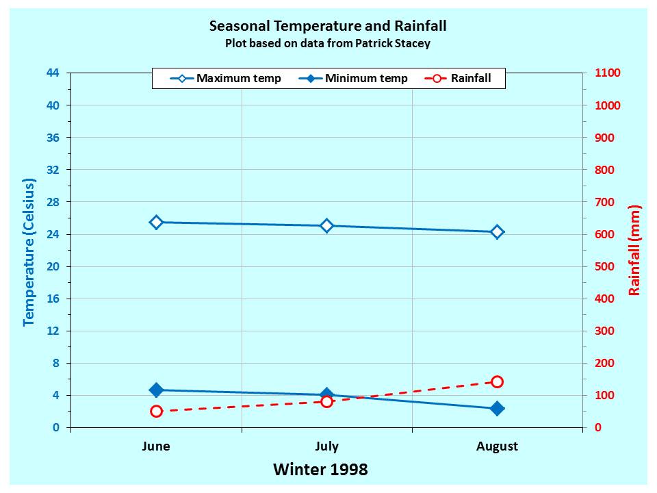
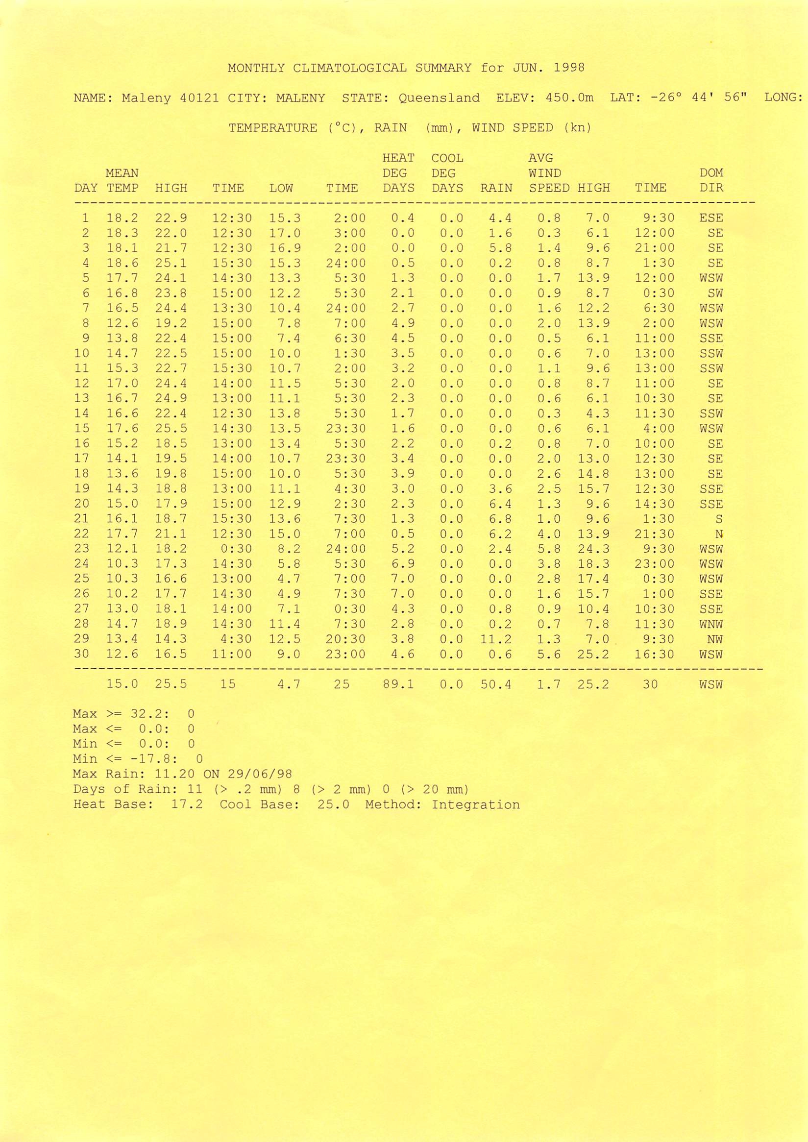

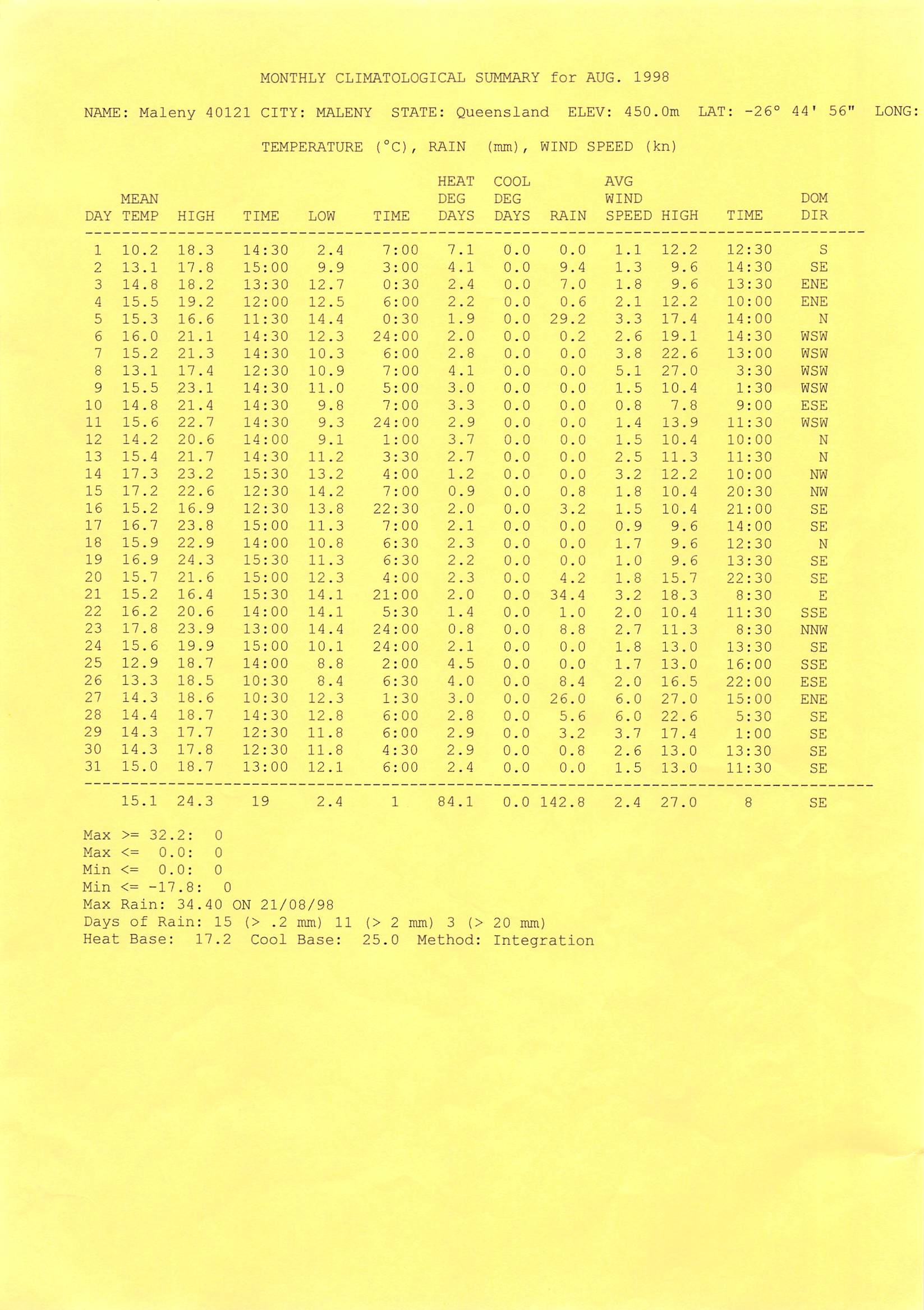
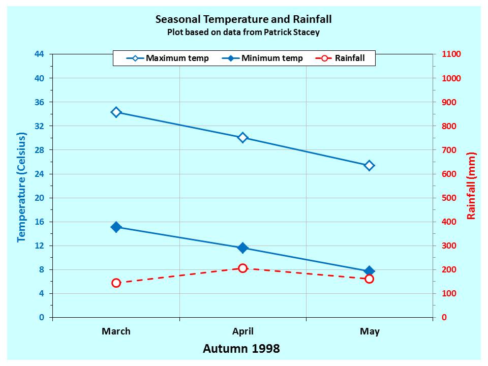
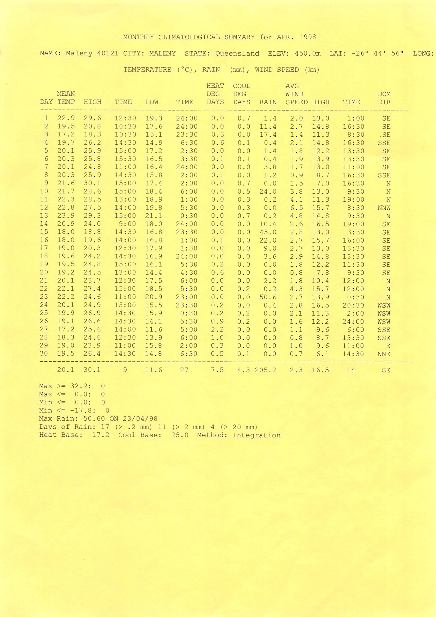
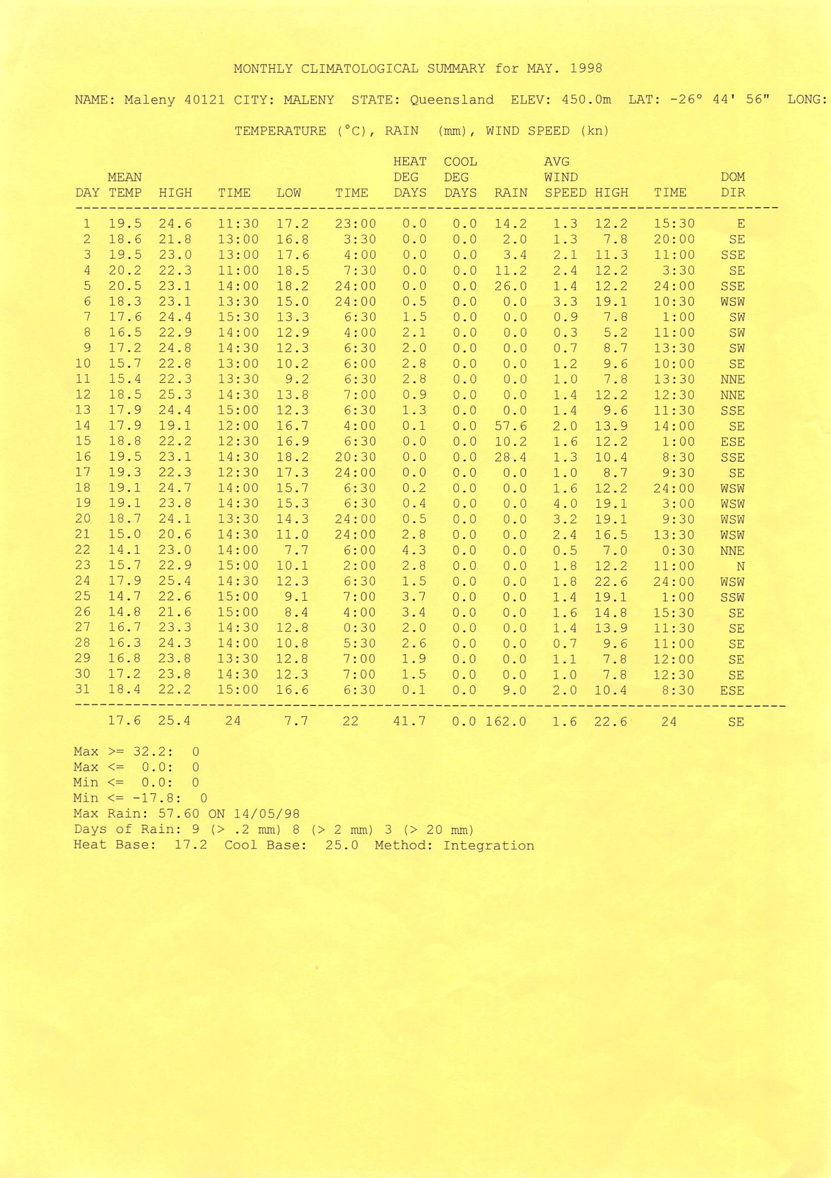
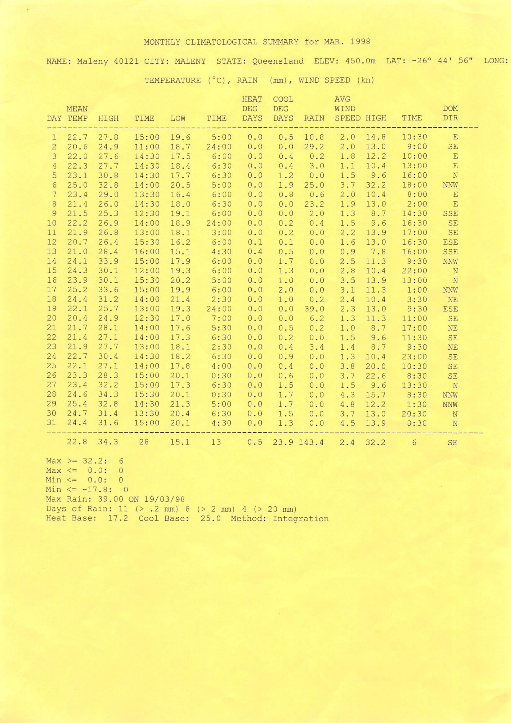
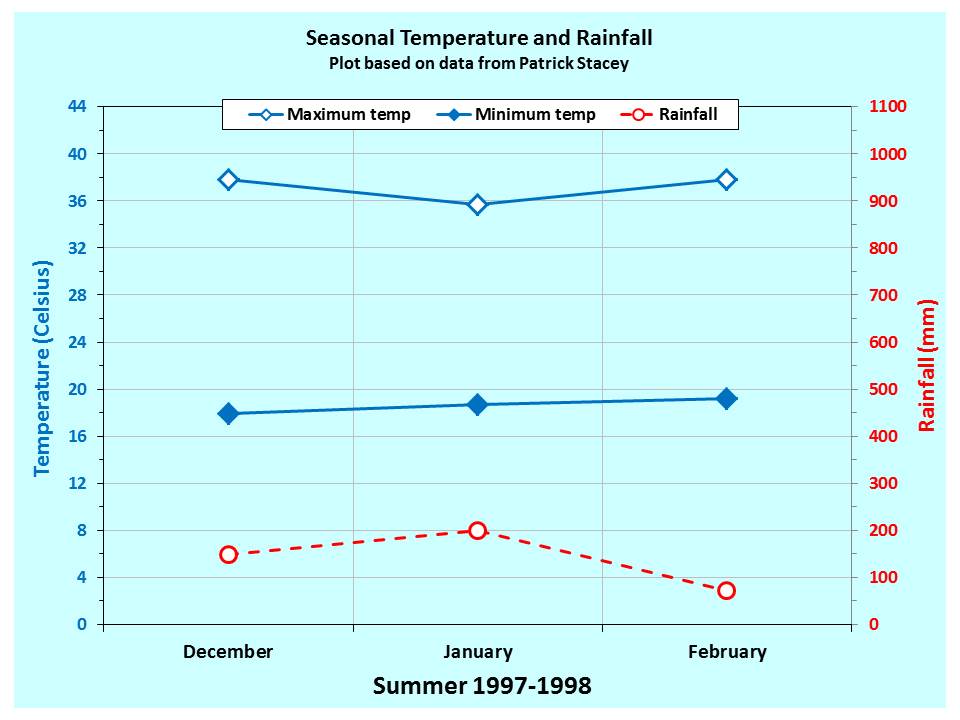
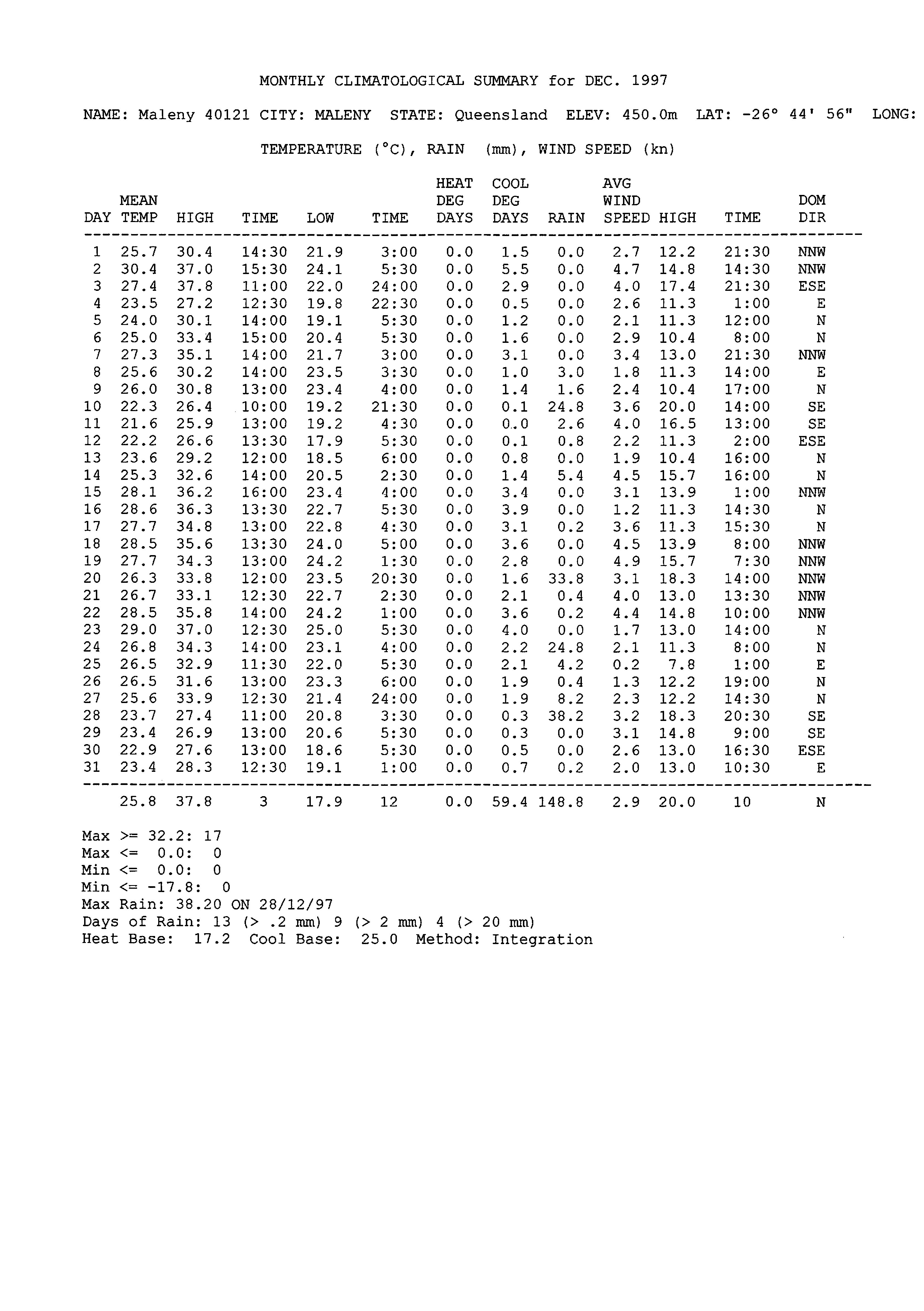
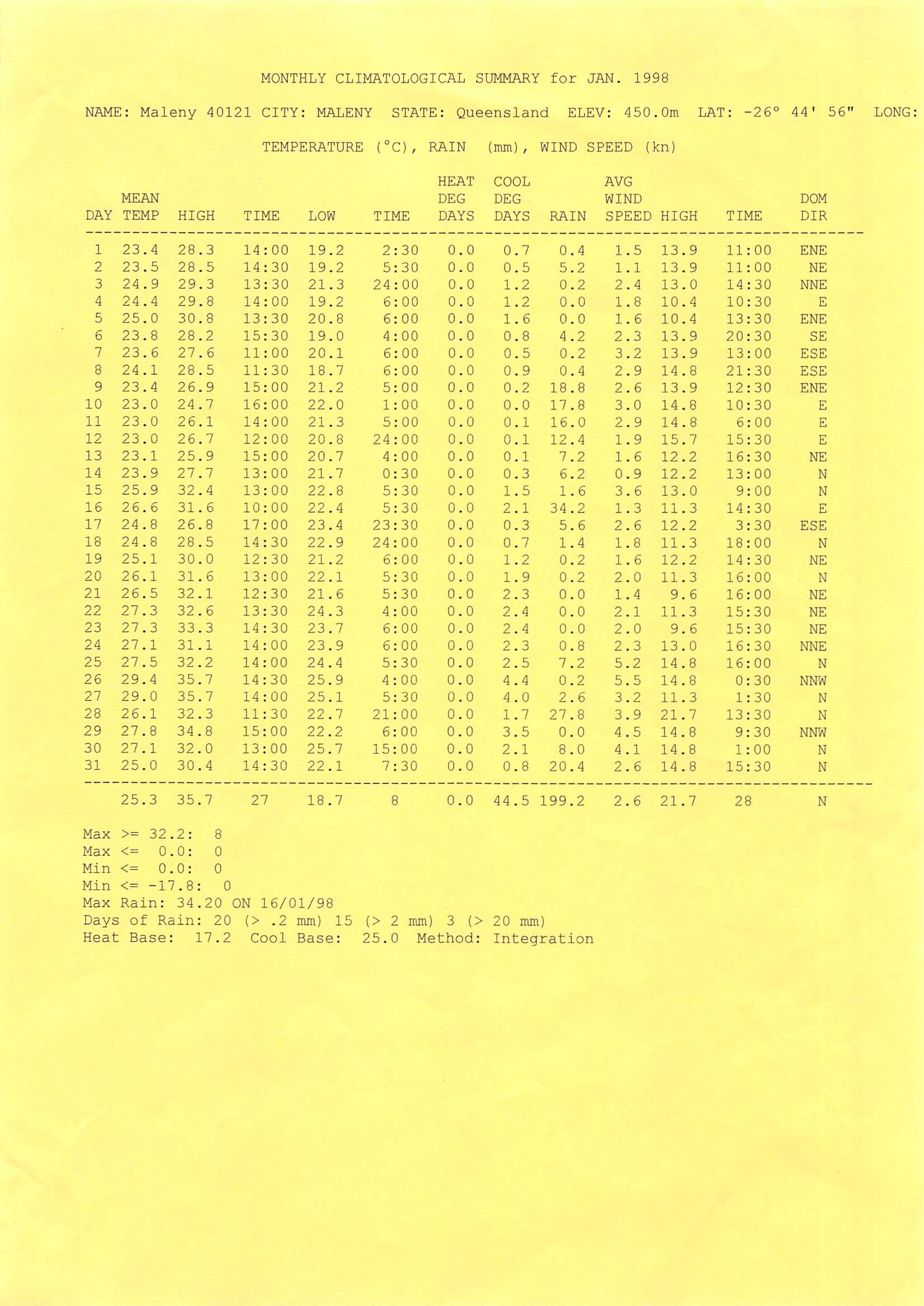
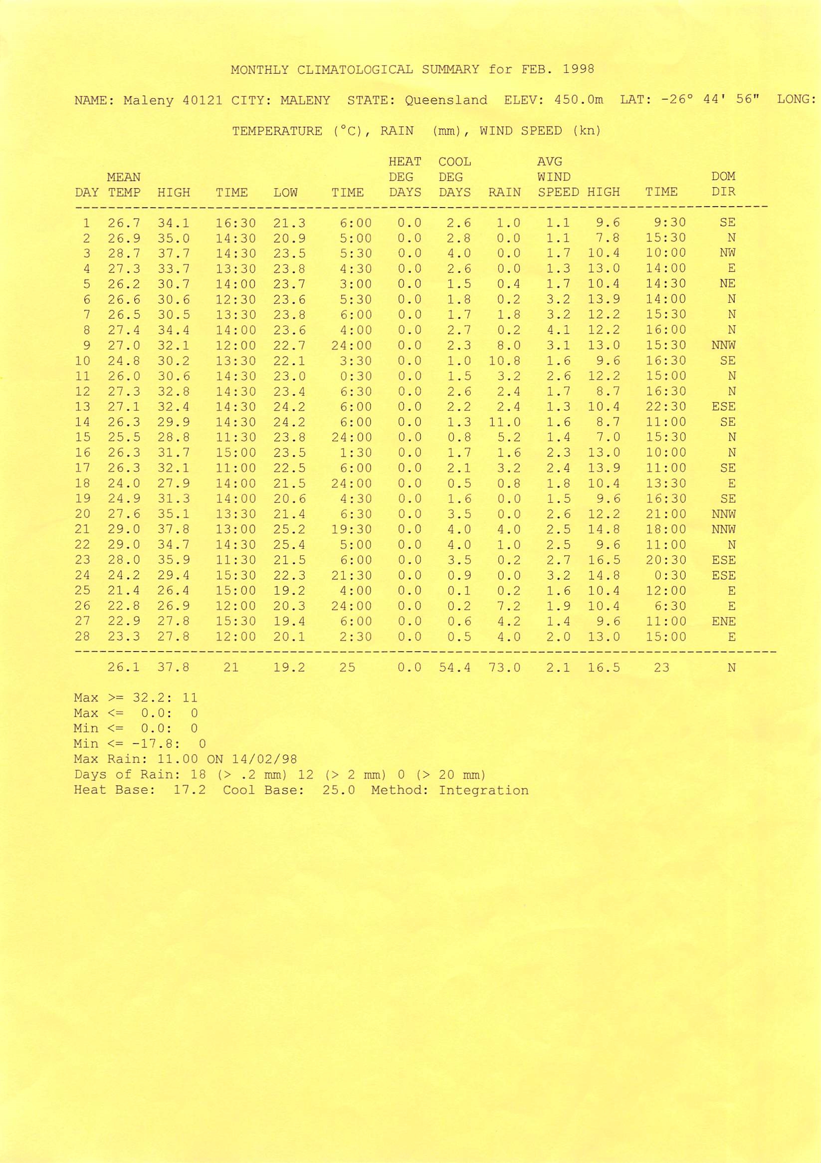
Maleny Apex have funded our scanner to digitise historical data

Hinterland Business Centre provide our domain malenyweather.com